Map View

There are two forms of map view showing two types of projection, namely Plate Carrée and Mercator. For more information on these projections see:

http://en.wikipedia.org/wiki/Map_projections

These views can be zoomed and panned using the move by:

• To move the map: click the left mouse button and while held down move the move
• To zoom the map in and out: use the mouse scroll wheel

There are a number of mouse “modes”, including:

Default mode – mouse moves the map

Station move mode – mouse used to move stations

Zoom mode – mouse used to select area to zoom into

Terrain mode – mouse used to select area to load terrain region (see Modules User Guide)

Path profile mode – mouse used to create new path profile (see Modules User Guide)

Move path profile mode – mouse used to move any of the path profile start or end points (see Modules User Guide)

Land Use mode – mouse used to select area to land use terrain region (see Modules User Guide)

Selecting Properties from the View menu (with a Map window active) or button from the toolbar brings up the Edit Map View dialog.

The properties dialog is also one of the options on the pop-up menu that can be accessed by right clicking on the map, as shown below:

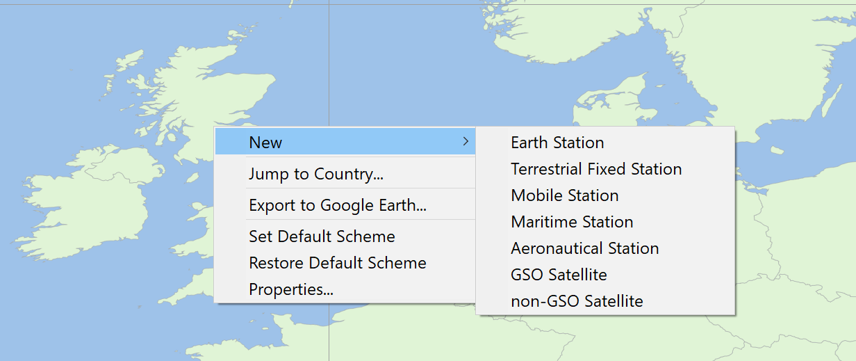
Note a slightly different menu will appear if you right click in locations where there is an Area Analysis, as discussed in Area Analysis Pop-Up Menu.

This menu can be used to:

• Create a new station at the position clicked
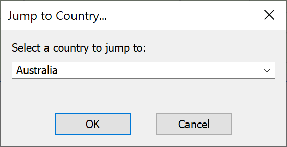
• Jump to a specific country as in the figure below:

• Export to Google Earth (as described in Interface to Google Earth)
• Set the current view configuration as the default one so that all new views of that type will open configured to look identical to the present one
• Restore Default Scheme: to change the configuration of the current view back to the default values
• Properties: this opens up the view properties dialog.

The view can be copied to clipboard using the Edit menu option or toolbar icon .

The map view properties dialog consists of five tabs:

• Features – the most regularly used features are presented in this tab
• Adornments & Behaviours – grids, titles and tick marks are defined here
• Overlays – here you can add Area Analyses, Terrain colours, Land use data and user defined bitmaps to enhance your output.
• Path Profiles
• Countries – schemes for colouring the map by country groups are defined here.

Each tab is described in the following sub-sections.

Features Tab

The General tab is shown below.

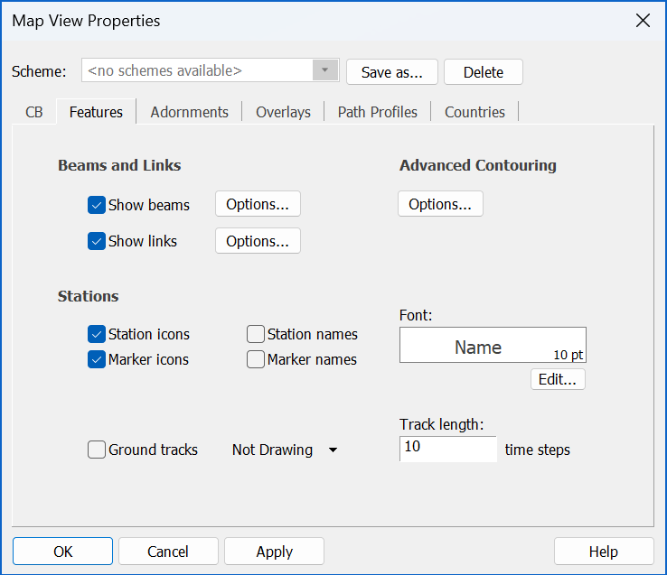
Switch the beam footprint and the Links on and off by checking or unchecking the boxes. The options buttons allow you to change the display properties.

Beam Options

To change the beam display options, click the options button next to “Show beams”. This will bring up the beam display options dialog (shown below).

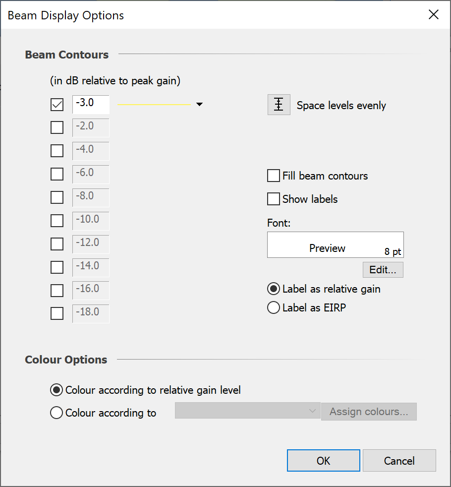
The dialog is split into two sections. The first section allows you to specify the footprints you want to display and their relative gain levels. Line styles can be selected for each beam contour that is being displayed.

If you want to display several footprints between two relative gain levels, set the top and bottom contour levels to the extreme values and click “Space Levels Evenly” to automatically set the levels for the footprints in between.

There is an option for filling the beam footprints with the line colour. Label display and formatting is also user definable.

The “Colour Options” section allows you to choose how the beam footprints are coloured when displayed on the map view.

The default option allows you to colour each footprint according to its relative gain level. Clicking next to the box where the level is set, sets the colour and line style.

The other option is to colour beams according to the Station Group, Station, or Antenna that they belong to.

To choose which one of these you want to colour by, select the ‘Colour according to’ radio button and click on the drop-down box activated next to the button.

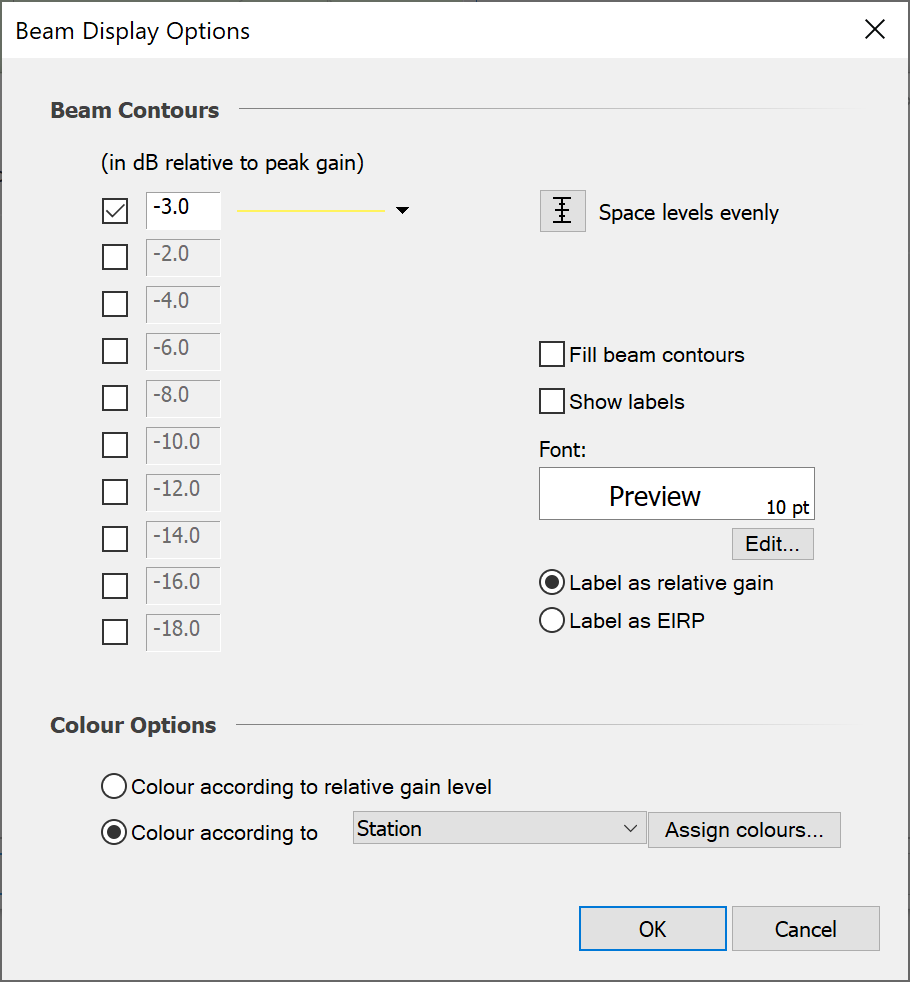
The levels are still set at the top of the dialog. However, the colours are assigned according to the Group / Station / Antenna / Antenna Type.

To change the colours associated with each Station Group, Station, Antenna, Antenna type, click Assign Colours. This will open the Assign Beam Colours dialog.

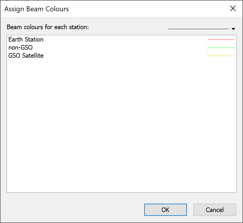
This dialog allows you to navigate to the objects you have chosen to colour by and select a colour and line style to apply to the beams.

Link Display Options

To change the link display options, click the Options button next to Show links. This will bring up the Link Display Options dialog (shown below).

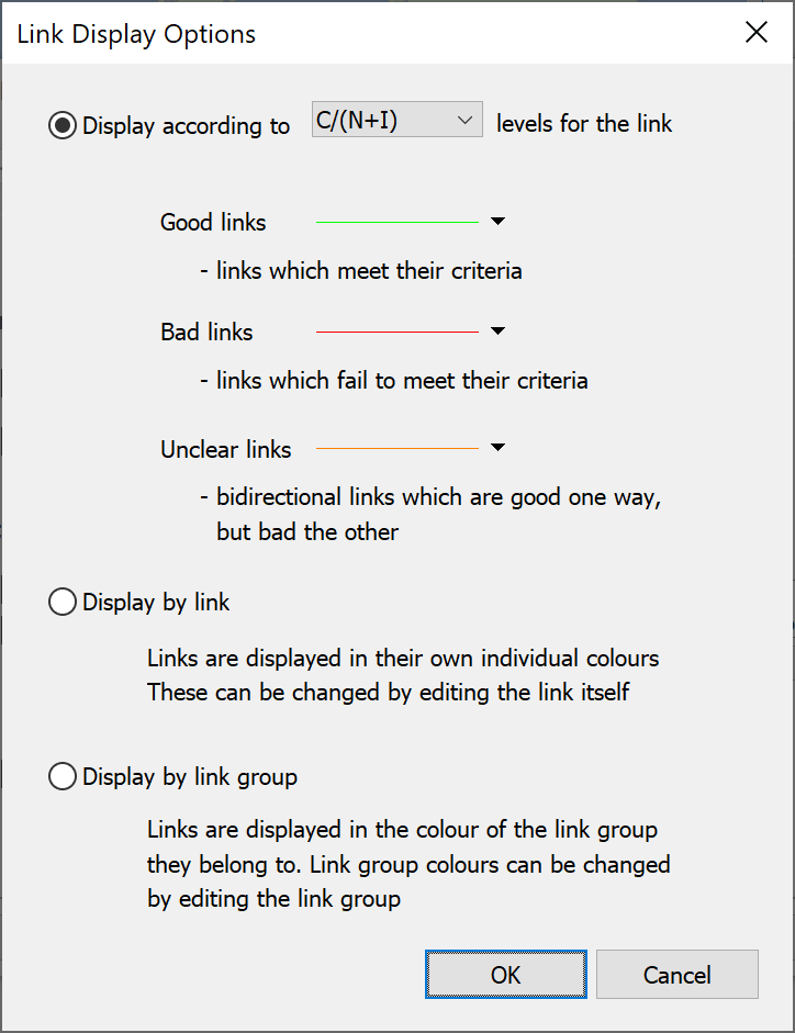
There are three options. You can display links according to one of the interference parameters (I, I/N, C/(N+I) etc.). The interference parameter is chosen from the drop-down list. You can then choose the colours for good, bad and unclear links.

The other two options allow you to display the links in their own colours or in the colours of the link group. These colours are set by editing the individual Links and Link Groups themselves.

Station Options

Station names can be switched on and off for normal stations and for marker stations. The font can be set as well. All fonts will now be displayed at the font size you choose.

Station ground track length can now be set on the dialog – note that this track length is applied to all map and 3D views. Colour and line style are set using the new line style control. There is also an option to set the track colour from the station colour.

Advanced Contouring

This option can be used to produce contours that show how link and station variables change over an area. For example it could show contours of where the interfering signal strength reaches a certain level.

As this is similar to the Area Analysis it is described further in Advanced Contouring using Groups.

Adornments & Behaviours

Adornments can be added to the view to explain what is being displayed or to enhance its appearance. The dialog is shown below.

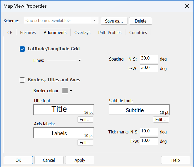
There are two sections to the adornments tab. The first deals with the latitude/longitude grid and the second deals with borders titles and axes.

Latitude/Longitude Grid

You can show or hide the latitude/longitude grid by ticking the check box at the top left of this tab. You can also set the line style for the grid lines. The grid size is defined by latitude and longitude spacing – type the number of degrees you want between each grid line in the boxes on the right-hand side of the dialog

Border, Title and Axes

If you switch this option on, a border will appear around the map area. You can change the colour of the border by clicking in the colour box.

The view title and subtitle are displayed in the centre of the top part of the border. Labels are shown along the latitude and longitude axes. You can set the spacing for tick marks on these axes. The fonts for all these can be adjusted.

When all the adornment options are switched on, the view will look something like the one below.

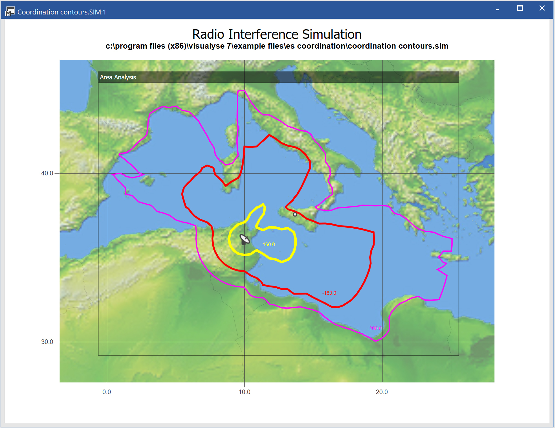
Show Scale Bar

Enabling this option shows a Scale Bar on the Map View.

Zoom at Cursor

Enabling this option make the mouse wheel zoom at the cursor location

Overlays

The overlays tab allows you to add features to a map which will enhance your output aesthetically and can also add a large amount of easily digestible information.

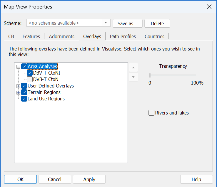
Overlays fall into four categories:

1. Area Analysis – any analyses produced so far in the simulation can be overlaid on all views
2. Terrain regions – if terrain data are included they can be selectively displayed as a colour coded overlay
3. Land Use Regions – used in the determination of clutter loss, Land Use data can also be displayed as colour coded overlays.
4. Overlays – allows you to add additional information onto the view including point, vector, and raster data, as explained below

Types of Overlay

There are four types of user defined overlay, namely: point, vector, drawing objects and raster data. The required file formats for all overlays are described in the Technical Annex.

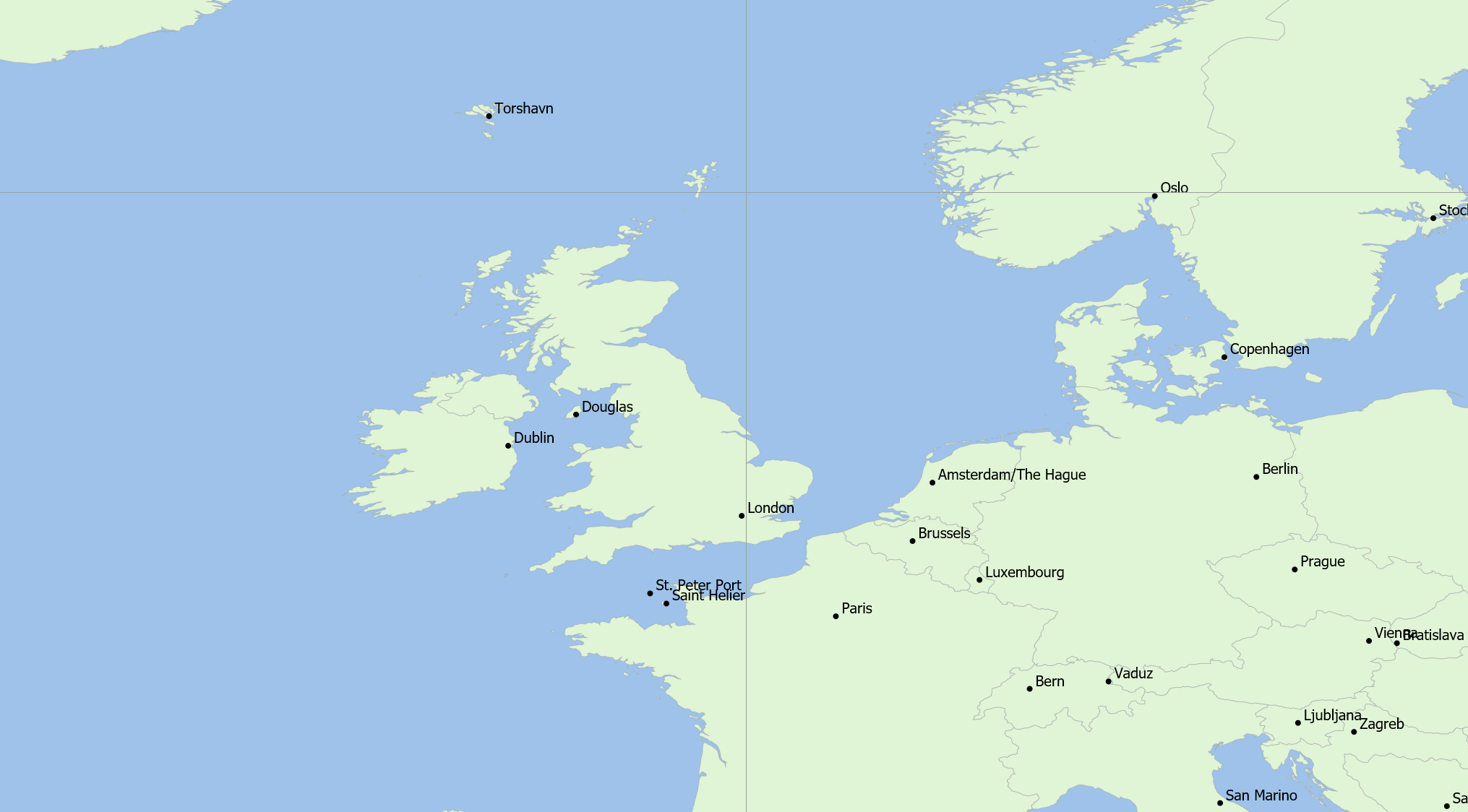
Point data allows specific locations to be marked and given a label. An example of point data is the user defined overlay “Capital Cities of the World”, as in the figure below:

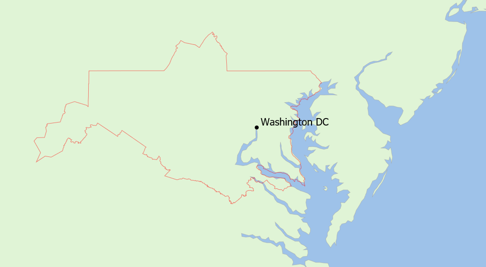
Vector data allows lines to be drawn at specific locations: this could be to show roads, railways, or borders. An example of vector data is the boundary of the Washington BEA licence as shown in the figure below.

Drawing objects allows simple shapes (rectangles, ellipses and grids) to be drawn at specific locations.

Raster data is graphical data such as maps but could include images of (say) population density or other information. These can cover the entire Earth or just a small part, defined using a rectangle. The example below shows a map from the Ordnance Survey (OS) in the UK overlaid on the Mercator view:

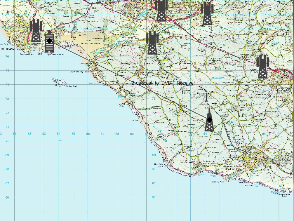
Note that raster data will have been generated assuming a specific projection and therefore care should be taken when displaying on either the Plate Carrée or Mercator view to ensure it is appropriate. The 3D view works like a Plate Carrée at large scale (i.e. the whole Earth) and Mercator and small scale (zoomed far in). Vector and point user defined overlays will work in any projection.

Adding an Overlay

The overlays tree lists everything Visualyse Interplanetary knows about, and the check boxes choose which of those items a particular view shows. Overlay files of your own can be added to that tree.

To add an overlay:

1. Click “Add...” underneath the overlays tree. The same option appears if you right click the tree, in which case the new overlay is filed under the branch or group you clicked.
2. Select the overlay file. Visualyse Interplanetary reads XML, KML, KMZ and shapefile overlays.
3. Give the overlay a name in the Add External Overlay dialog and click OK.

The overlay is added to the “Overlays” branch, ticked so that it appears in the view being edited, with its properties shown to the right of the tree. Overlays you have added are marked in the tree to set them apart from those supplied with Visualyse Interplanetary.

An overlay you add belongs to Visualyse Interplanetary rather than to one view. It is offered in the overlays tree of every map view and 3D view, and it is still there the next time Visualyse Interplanetary is started. Only the check box and the display properties are held per view. A file can only be added once. Choosing a file that is already in use reports which overlay uses it. Files held in the built in overlays folder are loaded for you, so they cannot be added again.

Naming and Grouping Overlays

An overlay name has to be unique. As you type in the Add External Overlay dialog a message appears beside “Name:” if the name cannot be used, and OK stays unavailable until it is acceptable.

The name can also place the overlay in a group. Use a backslash to separate the group from the overlay, so that “Grids\France” shows an overlay “France” inside a “Grids” group. A forward slash can be used instead. Groups can be nested up to three levels deep. Ticking a group ticks every overlay within it, and a group only some of whose overlays are ticked is shown part ticked.

To rename an overlay afterwards, select it and click “Edit” beside its name. Every view’s record of the overlay is updated with it.

Overlay Properties

Selecting an overlay in the tree fills the panel to the right of it with that overlay’s properties. Which of them appear depends on the kind of overlay selected, and everything apart from the name and the file location belongs to the view being edited, so the same overlay can be drawn differently in each view that shows it.

• Name – the overlay’s own name, without the groups it sits in. Click “Edit” to change it
• Transparency – how much of the layers beneath shows through this one
• Colour – the marker colour, for a point overlay
• Outline – the colour, line style and thickness, for a vector or drawing overlay
• Show labels – whether labels are drawn in this view, offered for an overlay whose data carry label text
• Font – the font, size and colour used for those labels. The box previews the current font and “Edit...” opens the font dialog. The font can only be changed while “Show labels” is ticked
• File location – the file the overlay is read from. It cannot be typed into. Click “Edit...” to point the overlay at a different file

The name and file location of an overlay supplied with Visualyse Interplanetary cannot be changed, so neither is offered for one. For an Area Analysis, a terrain region or a land use region, only the transparency applies.

Deleting an Overlay

To remove one of your own overlays, select it and click “Delete” underneath the tree, or right click it and choose “Delete”. This takes the overlay out of Visualyse Interplanetary altogether, so it leaves the overlays tree of every view and not just the one being edited. Only overlays you have added can be deleted here.

Adding, renaming, relocating and deleting all take effect at once, but closing the map view properties dialog with Cancel reverses them, so an overlay removed by mistake can be reinstated that way.

Overlays that Cannot be Loaded

An overlay file is read only when the overlay is needed, so a file that has been moved, renamed, deleted or damaged since the overlay was added is not found out about until then. Visualyse Interplanetary marks the overlay in the tree with a warning symbol and replaces the display properties with the reason and the file location it expected, together with one of two buttons:

• “Locate...” – offered when the file cannot be found. It opens a file browser at the folder the overlay was added from, or the nearest folder above it that still exists, with the original file name filled in. Choose the file in its new home and the overlay is tied to it again
• “Retry loading” – offered when the file is present but could not be read. Correct the file, then click it to read the file again

If the file chosen when locating an overlay goes under a different name, you are asked to confirm that the two belong together before they are tied. A file that already backs another overlay is refused.

Failures are gathered together and reported once, in the Overlay Load Error dialog, which names each overlay concerned and gives the reason for it. Click “Fix Now...” to go straight to the Overlays tab with the first of them selected, ready to be located or read again, or OK to attend to it later. Each overlay is reported only once in a session.

Managing What is Displayed

The four types of user defined overlay, together with the Area Analysis, terrain and land use overlays, mean that there is a lot of information that could be displayed on either of the map views or the 3D view. Indeed typically the key issue is how to select and configure what is shown.

A number of controls can be used to manage what is shown on the views, including:

• Check boxes to show or hide each of the items
• Controls to change the order in which each layer is display
• Controls to change the degree of transparency from one layer to the layers below

The final image is built up by adding each layer on top of the other with the degree of transparency as requested.

The result of combining these three layers is a composite in which the graphics are merged so that lower layer information can be seen due to the transparency of the higher layers.

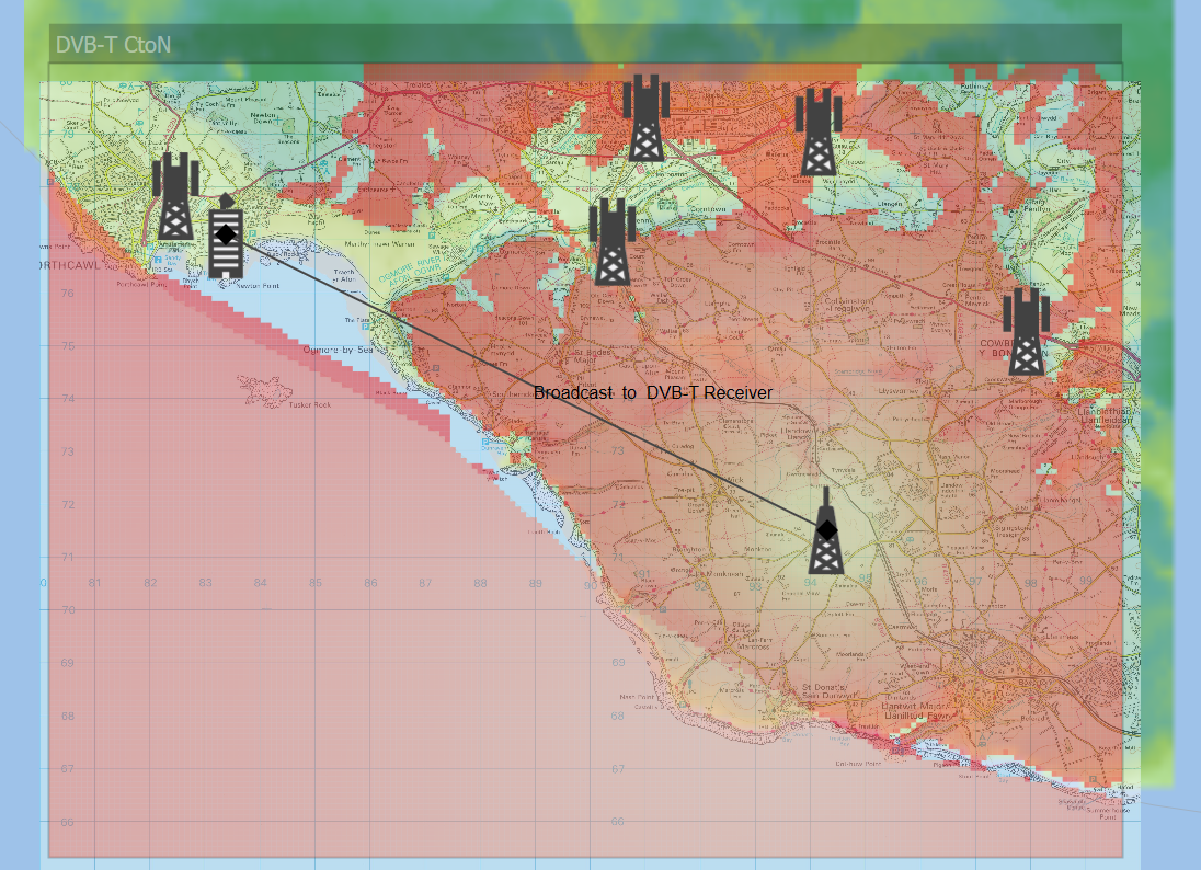
The arrow keys on the View Properties Overlay’s tab can be used to move the position of:

• An overlay category (e.g. Area Analyses, Terrain Regions, Land Use Regions, Overlays) with respect to another overlay category
• An overlay with respect to other overlays within that particular overlay category

Select the item of interest (category or overlay) then click on the up or down arrow as required. Hold CTRL while clicking to move the item ten places at a time. The arrows show a double head while CTRL is held.

To change the level of opacity (and hence its transparency) of an overlay, select it and then click on the Transparency control, as in the figure below.

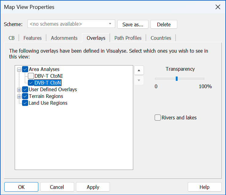
The following should be noted:

• It is easy to overload the view with too many overlays: select the ones you want and hide others
• The most important overlays should be highest on the list and less important ones lower down
• The level of transparency of each overlay can be used to show more or less of the lower layers

Tip: Colours of terrain and land use pixels can be selected to avoid clashing with other overlays. For example if an area analysis of coverage from a base station uses green and yellow to plot signal strength, select different colours to show the terrain heights or land use codes.

Path Profiles

Where terrain path profile views have been created, they are indicated on map views as a coloured line. The Path Profiles dialog lets you control how that line, and any text associated with it, is displayed.

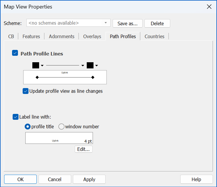
Countries

The final tab on the Map View Properties dialog is the Countries tab. This allows you to set the display options for the country polygons in the map.

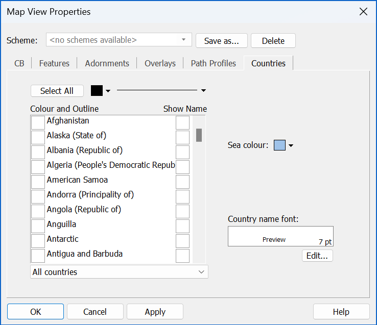
The main function of this tab is to allow you to set the colours and outlines of the countries on the map. A list of all the countries is displayed on the left-hand side of the dialog. Each country has a coloured square next to it. This represents the colour and outline that will be used to display that country.

To change a country’s colour, first select it in the list. At the top of the list are two controls one to select the colour and one to set the outline.

When you change the colour or line-style, these will be set for the selected country. If you want to set these colours for another country, first select the new country. Now all you need to do is click the colour or outline button itself (not the drop-down) and that colour or style will be applied.

You can change more than one country at once by applying colours and styles to a multiple selection. You can also click the Colour All button to apply the current colours to all the countries in the list.

At the bottom of the list is a drop-down that allows you to show only certain groups of countries. Examples are - All countries, Continents and ITU regions. Having selected a group, you could apply colours to all countries in the group.

As well as country colours, you can select whether to show US state borders or rivers and lakes. You can also choose the sea colour.

Choose whether you want to show country names. The font can be set for these as before. However, fonts will now be displayed at their actual point size.