Link Budget Calculations

• Power Calculation Reference Points
• Noise Calculation
• Other Parameters
• PFD and Field Strength
• Interference Adjustments
• Link Group Calculations
• Modelling Radar Reflections
• Listen before transmit

Power Calculation Reference Points

In order to be able to model a wide range of radio systems a generic link model is used in all calculations in Visualyse Professional. The basic link budget is as follows:

$${\mathrm{C}}_{\mathrm{RX}}={\mathrm{P}}_{TX}+{\text{ GPeak }}_{TX}+{\mathrm{GRel}}_{TX}-L_P+{\text{ GPeak }}_{RX}+{\text{ GRel }}_{RX}-L_{RX}$$

Where:

$P_{TX}=$ transmit power at input to antenna (dBW)

GPeak ${}_{\mathrm{TX}}=$ transmit antenna peak gain $(\mathrm{dBi})$

GRel ${}_{Tx}=$ transmit antenna gain towards the receiver relative to peak (dB)

$L_P=$ propagation loss between transmit and receive antennas (dB)

GPeak ${}_{\mathrm{Rx}}=$ receive antenna peak gain $(\mathrm{dBi})$

GRel ${}_{\mathrm{Rx}}=$ receive antenna gain towards the transmitter relative to peak $(\mathrm{dB})$

$L_{RX}=$ losses between receive antenna and input to the receiver $(\mathrm{dB})$

The reference points are therefore:

Transmitter: at the input to the antenna

Receiver: at the input to the receiver

Hence there is no field in Visualyse Professional for the transmit line loss.

The reference points for the link budgets are therefore as shown in the figure below:

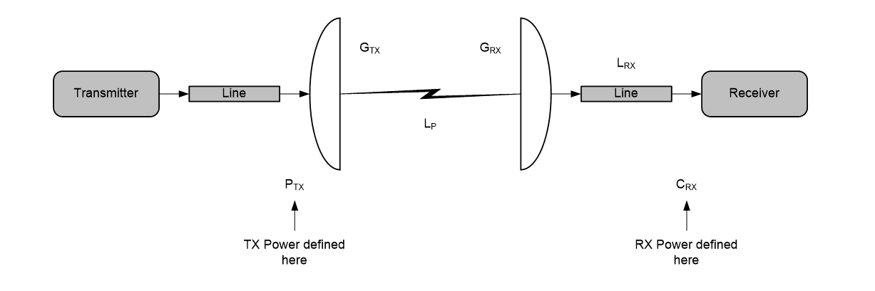
Note that:

$$\begin{array}{rl}& {\mathrm{G}}_{\mathrm{TX}}={\mathrm{GPeak}}_{\mathrm{TX}}+{\mathrm{GRel}}_{\mathrm{TX}}\\ & {\mathrm{G}}_{\mathrm{RX}}={\mathrm{GPeak}}_{\mathrm{RX}}+{\mathrm{GRel}}_{\mathrm{RX}}\end{array}$$

The receive measurement point can be made to be at the output of the receive antenna by setting the LRX to zero.

Noise Calculation

In Visualyse Professional there are two ways to define the noise at the receiver:

• Enter the noise temperature of the receiver directly
• Allow Visualyse Professional to calculate the receiver noise temperature from the various components.

The calculation of receiver input noise is based upon the following parameters:

The system temperature is calculated from:

$$T_{\text{sys }}=\frac{T_{\text{ant }}}{L_{\text{feed }}}+T_{\text{feed }}\left(1-\frac{1}{L_{\text{feed }}}\right)+T_{rx}$$

Where:

${\mathrm{F}}_{\mathrm{rx}}=$ noise figure of receiver

${\mathrm{T}}_{\text{ant }}=$ noise temperature of antenna

${\mathrm{L}}_{\text{feed }}=$ feeder loss

${\mathrm{T}}_{\text{feed }}=$ feeder temperature

$T_{rx}=\left(F_{rx}-1\right)\ast T_{ref}$ where $T_{ref}$ is 290 Kelvin

Converted to noise spectral density this is:

$$N_{\text{sys }}=k+10{\log }_{10}T\text{ where }\mathrm{k}=-228.6\text{ is Boltzman’s constant in }\mathrm{dB}$$

Other Parameters

There is a wide variety of methods to define link budgets and these can use different parameters that might need to be mapped onto Visualyse Professional fields.

• Transmitter losses: losses such as transmit link losses can be modelled by reducing the transmit power accordingly.
• G/T: Some antennas have their performance defined via their G/T. In this case it is necessary to determine separate G and T figures to be entered into the link budget above.
• Pointing losses: At the transmit side these can be modelled either by reducing the transmit power according to the required level of pointing loss or by adding a slight offset to the antenna pointing angles. At the receive side the pointing loss could be modelled as either being part of the receiver losses or adding a slight offset to the antenna pointing angles.
• Polarisation losses: These can be included by either adding them to the receive feed loss or adjusting the required C/N or C/(N+I) threshold upwards.
• Baseband losses: losses such as implementation losses, demodulation margin etc can be modelled by adjustment of the threshold required.

PFD and Field Strength

In Visualyse Professional the PFD calculation assumes free space path loss, hence it is simply:

$$pfd=\frac{EIRP}{4\cdot \pi \cdot d^2}$$

It is sometimes useful to derive the PFD assuming the other propagation models within Visualyse Professional’s library. In this case it is possible to calculate the signal (wanted or interfering) as received at an isotropic receiver and convert into either PFD or field strength.

The conversion factors in the case of interference is:

$$pfd=I+10\log \left[\frac{4.\pi }{{\lambda }^2}\right]$$

Note that $\mathrm{c}=\mathrm{f}\lambda$ and that $\mathrm{c}=2.997\mathrm{e}8\mathrm{m}/\mathrm{s}$

To convert the pfd into field strength use:

$$\text{ Field strength }\mathrm{dB}\mu \mathrm{V}/\mathrm{m}=\mathrm{pfd}+145.8$$

Interference Adjustments

• Carrier Overlap
• Frequency Overlap
• Interference Calculation Adjustment
• Frequency Dependent Adjustment
• Polarisation Adjustment
• Mask Integration to derive NFD

Carrier Overlap

It should be noted that all unless masks are given, carrier spectre are assumed to be square with the following parameters defined:

• Central frequency
• Occupied bandwidth
• Allocated bandwidth

Typically the wanted and interfering signals have different central frequencies and / or bandwidths. It is therefore necessary to consider how to adjust the interference calculation to take account of bandwidth factors. The figure below shows a typical situation:

The overlap algorithm is:

$$\begin{array}{rl}& {\text{ Start }}_A={\text{ Freq }}_A-{\mathrm{OBW}}_{\mathrm{A}}/2\\ & {\text{ End }}_A={\text{ Freq }}_A+{\mathrm{OBW}}_{\mathrm{A}}/2\\ & {\text{ Start }}_B={\text{ Freq }}_B-{\mathrm{OBW}}_B/2\\ & {\text{ End }}_B={\text{ Freq }}_B+{\mathrm{OBW}}_B/2\end{array}$$

Then using the start and end frequencies above:

$$\begin{array}{rl}& \text{ StartOverlap }=\max \left({\text{ Start }}_A,{\text{ Start }}_{\mathrm{B}}\right)\\ & \text{ EndOverlap }=\min \left({\text{ End }}_A,{\text{ End }}_{\mathrm{B}}\right)\end{array}$$

So:

$$\text{ Overlap = EndOverlap }-\text{ StartOverlap }$$

This is used in the two bandwidth calculations: whether to include the carrier as being partially co-frequency and how much energy from the interfering carrier to include.

Frequency Overlap

An interfering carrier is included in the interference calculation if at least one of the following is true:

• the overlap between carriers (as calculated above) is greater than zero
• the force co-frequency flag is set

Interference Calculation Adjustment

If there is overlap between two carriers, then it is necessary to determine how much energy to include. Three alternatives are available, and the result is the BWF factor which is used to multiply the interfering carrier level to get the resulting interfering level I.

No Adjustment

In this case the BWF is always 1.

Spectral Power Density

In this case the ratio of the two is used, based on the power spectral density:

$$\text{BWF}=\frac{OB{W}_W}{OB{W}_I}$$

Overlap

In this case the extent of overlap is used, calculated using:

$$\text{BWF}=\frac{\text{ Overlap }(\text{ Carrier }W,\text{ CarrierI })}{{\mathrm{OBW}}_I}$$

Note that for the force co-frequency case the frequency of both carriers is set to the same and ${\mathrm{OBW}}_{\mathrm{W}}\le {\mathrm{OBW}}_1$, and so this becomes the same as Spectral Power Density.

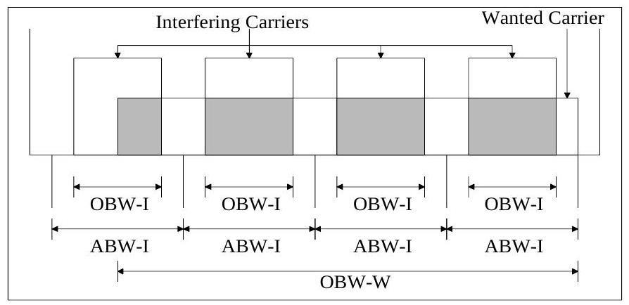
Multiple Carriers

In this case it is assumed that there could be multiple interfering carriers in the bandwidth of the wanted signal. Each interfering carrier is separated by its ABW, but occupies only the OBW. This is shown in the figure below:

Figure Multiple Interferers Into Wanted Carrier

The calculation is therefore:

Frequency Dependent Adjustment

The bandwidth adjustment in the tables above is based upon rectangular blocks of frequency. Some carriers are shaped, such as TV, and so the interference to/from one of these carriers will depend on the separation between central frequencies.

This can be included in the link calculation using a table of advantage vs offset of central frequencies. Linear interpolation is used between entries in the table, with no extrapolation at the ends of the table.

Polarisation Adjustment

Polarisation adjustment can be done one of three ways:

1. no adjustment
2. standard ITU adjustment table
3. user defined table

The tables give constant adjustments based on wanted and interfering carrier polarisations. The user defined table allows checking for main beam to main beam alignment. This occurs when the transmit and receive relative gains are -3 dB or higher.

Note that it is possible in Visualyse Professional to do full cross-polar gain pattern calculations by entering the cross-polar values for one system (typically interfering) and using the co-polar gain pattern for the other system (typically wanted). This can be done using the table patterns.

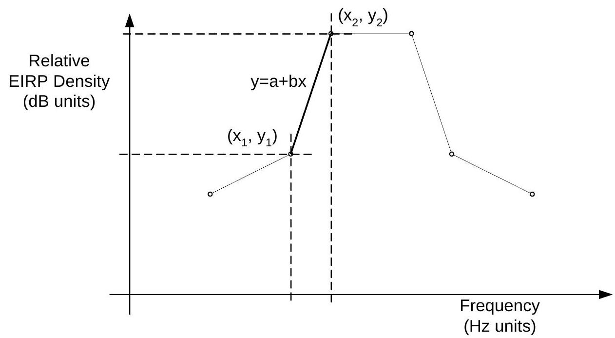
Mask Integration to derive NFD

In Visualyse Professional it is possible to specify the following two masks:

1. The transmit mask is defined as the relative power density compared to in-band: in other words as a table it would be defined in dB while in the integration the units would be an absolute ratio.
2. The receive mask is defined as the relative attenuation of the receive signal compared to in-band: in other words as a table it would be defined in dB while in the integration the units would be an absolute ratio.

Both the transmit and receive masks are defined using tables with linear interpolation in dB between each point and hence can be modelled as a set of straight lines with equation (in dBs):

$$\begin{array}{rl}& y_{tx}=a_{tx}+b_{tx}f\\ & y_{rx}=a_{rx}+b_{rx}f\end{array}$$

In which case the NFD is:

$$NFD=\sum _{f_{\min }}^{f_{\max }}NFD\left[f_1,f_2\right]$$

Where:

$$NFD\left[f_1,f_2\right]=\frac{10^P}{Q^{\prime }}\left(e^{Q^{\prime }{f}_2}-e^{Q{f}_1}\right)$$

And:

$$\begin{array}{rl}& P=\left(a_{tx}+a_{rx}\right)/10\\ & Q=\left(b_{tx}+b_{rx}\right)/10\\ & Q^{\prime }=\ln (10)\cdot \left(b_{tx}+b_{rx}\right)/10\end{array}$$

Note that in general the values of $a$ and $b$ are not user entered but are derived from a set of values at specific points, as in the figure below.

Three formats of this integration are available:

Integrate masks (Classic): Transmit and receive masks integrated and then divided by the transmit bandwidth. This is the correct approach if the TX spectrum mask is referenced to the mean in-band density i.e. 0 dB is when the power density = TX power / occupied bandwidth.

Integrate masks (NFD): Transmit and receive masks integrated and then divided by the integration of the transmit mask. This is the correct approach if the TX spectrum mask 0 dBi point is referenced to the peak power density.

Integrate masks (ETSI): Transmit and receive masks are integrated for the specified frequency offset and then divided by the integral of the TX and RX masks when co-frequency. This is the correct approach to be consistent with the methodology in ETSI TR 101 854 and is sometimes called the Frequency Dependent Rejection or FDR. To adjust for different bandwidth carriers the carrier overlap calculation is included in the adjustment as per Interference Calculation Adjustment.

Note on the ${\mathrm{HCM}}^1$ NFD: this is calculated as two terms, called NFD and MD where:

$$NFD=\frac{{\int }_{f_{\min }}^{f_{\max }}{M}_{TX}\left(f_{TX}\right)M_{RX}\left(f_{TX}\right)df}{{\int }_{f_{\min }}^{f_{\max }}{M}_{TX}\left(f_{TX}\right)M_{RX}\left(f_{RX}\right)df}$$

i.e. NFD $=10\log 10$ (OverlapAreaCoFrequency / OverlapAreaActualFrequency)

$$MD=\frac{M{I}_{TX}}{{\int }_{f_{\min }}^{f_{\max }}{M}_{TX}\left(f_{TX}\right)M_{RX}\left(f_{TX}\right)df}$$

Therefore the $\mathrm{MD}=10\log 10$ (TXArea / OverlapAreaCoFrequency)

Hence MD + NFD = 10log10(TXArea / OverlapAreaActualFrequency)

Therefore the total HCM bandwidth and mask integration factor is the same as the "Standard NFD" calculation described above.

Link Group Calculations

• Thermal Additional
• Wanted Signal Phase Addition

Thermal Additional

Thermal addition is used to calculate end to end performance for analogue systems. In this case the link qualities are added using the following formula:

$${\frac{C}{X}}_{dB}=10\log \left[\frac{1}{{\sum }_i\frac{1}{10^{\frac{\left(\frac{C}{X_{i,dB}}\right)}{10}}}}\right]$$

where X could be I, N or (N+I).

Wanted Signal Phase Addition

Some diversity systems use two links and merge the two received signals such that the wanted carriers remain in phase. This changes the phase of the interfering signal, and the following algorithm is used to add the link qualities (note in W not dBW):

$$\begin{array}{rl}& C_W=\sum _i{C}_{i,W}\\ & N_W=\sum _i{N}_{i,W}\\ & I_W=\left|I_{0,W}+\sum _i{I}_{i,W}\cos \varphi \right|\end{array}$$

where $\varphi$ is a random number between 0 and $2\pi$.

Modelling Radar Reflections

One of the most important uses of the electromagnetic spectrum is for radar.

When modelling radar in simulation tools the most important difference from most other types of radio system is that the signal is received after two paths via a passive reflection, as can be seen in the figures below:

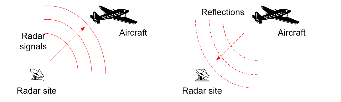
The signal strength that is received can be calculated using the standard radar equation (assuming free space path loss):

$$P_R=P_T{G}_T\frac{1}{4\pi R^2}\sigma \frac{1}{4\pi R^2}{A}_{eff}$$

Where:

$$\begin{array}{rl}& {\mathrm{P}}_{\mathrm{T}}=\text{ transmit power }\\ & {\mathrm{G}}_{\mathrm{T}}=\text{ transmit antenna gain }\\ & \mathrm{R}=\text{ range from radar to target }\\ & \sigma =\text{ radar cross section of the target }\\ & A_{\mathrm{eff}}=\text{ effective area of the radar receiving antenna }\\ & {\mathrm{P}}_{\mathrm{R}}=\text{ received signal }\end{array}$$

Radar reflections can be modelled via the Link’s End to Start power option. To enable this option:

• Create the radar station with antenna pointing at the aircraft
• Create the aircraft with the required height and for antenna use an isotropic gain pattern with gain 0 dBi
• Create a fixed or dynamic link with:
  • Start station = radar station
  • End station = aircraft
  • Start to End direction: set the transmit power of the antenna
  • End to Start direction: set the transmit power option to be “radar reflection” and then set the radar cross section to be that of the aircraft and the noise temperature to be that of the radar station, as in the example below:

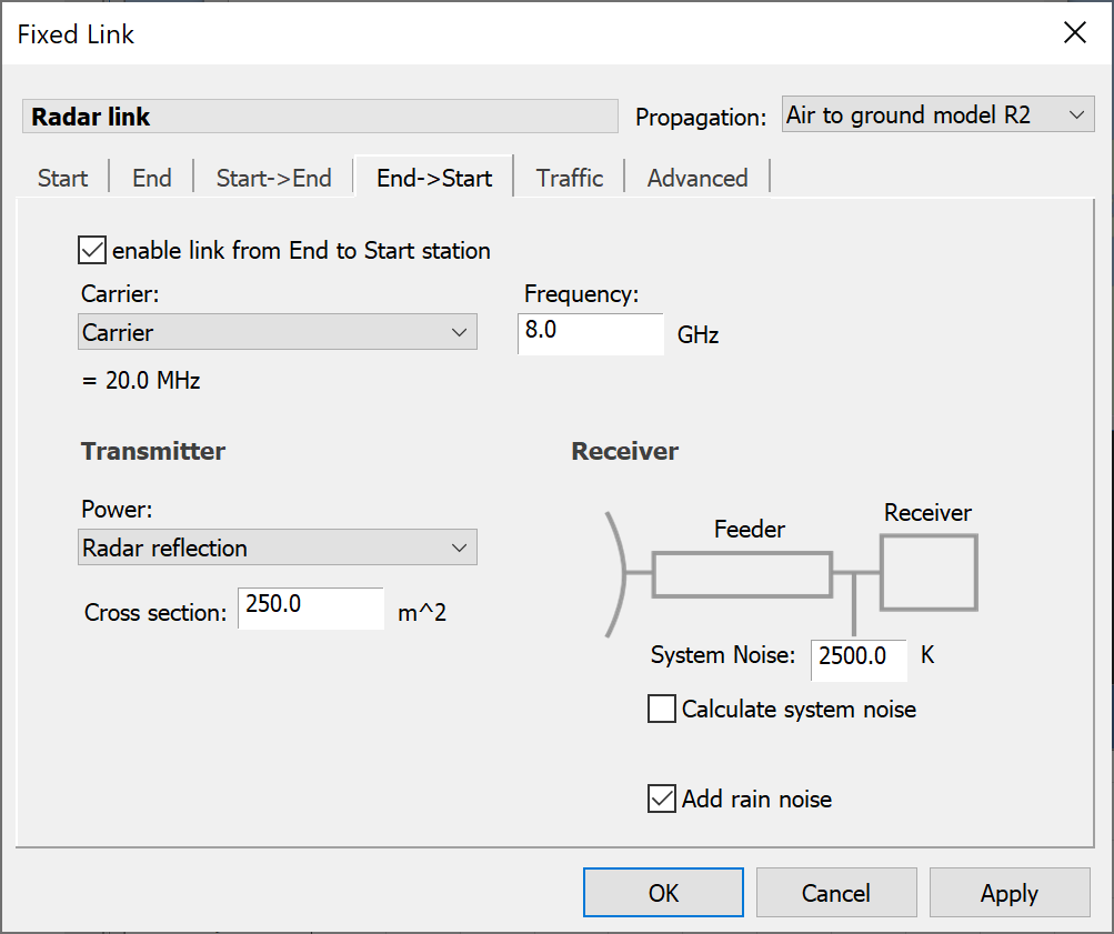
Having created this link the End to Start’s received power will be the radar station’s wanted signal.

Note that any propagation model could be used, not just free space path loss as in the equations above. In particular it could be appropriate to consider:

• Recommendation ITU-R P.452: this includes the effect of terrain and is considered acceptable for low altitudes
• Recommendation ITU-R P.528: this is designed for air to ground / ground to air links up to a maximum height of 20,000m. It does not include the effect of terrain

Both these propagation models can also include a percentage of time field.

Note that the following are checked by Visualyse Professional:

• The Endstart carrier must be the same as the StartEnd carrier
• The Endstart frequency must be the same as the StartEnd frequency
• The end station must use an isotropic antenna with gain = 0 dBi
• The Startend direction must be enabled

Listen before transmit

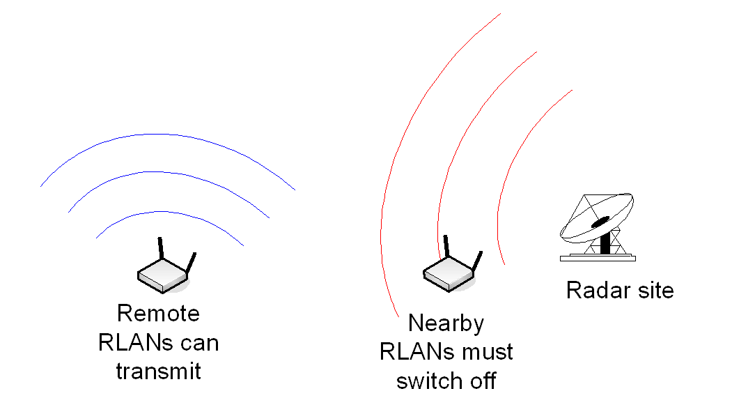
Recent developments of cognitive technologies, such as listen before transmit, are allowing a range of new sharing scenarios.

An example of this can be found in the 5 GHz band where Radio Local Area Networks (RLANs) can operate as long as they do not cause harmful interference into radars in the frequency ranges 5 250 - 5 350 and 5 470 - 5 725 MHz. The mechanism used to protect the radars is dynamic frequency selection based upon listen before transmit technologies.

As described in Recommendation ITU-R M. 1652, RLANs with the potential to transmit up to 200 mW e.i.r.p. must be capable of detecting radar signals of -62 dBm. If a signal is detected on a channel then it can not be used and instead the RLAN must try another channel.

This is shown graphically in the figure below:

In regulatory terms there could be a constraint similar to::

System A can only transmit at power = X if the signal received from System B is less than Y

The question is then, what are the relevant values of X and Y? This requires interference analysis taking into account deployment densities and propagation conditions.

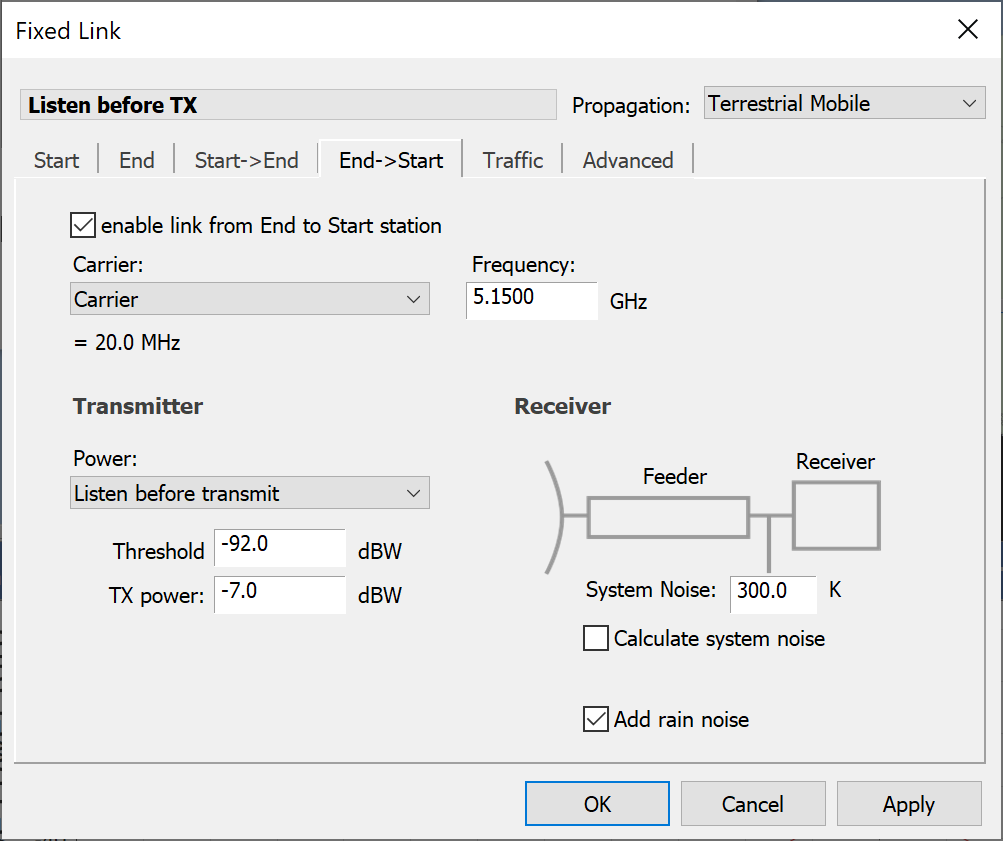
This can now be modelled in Visualyse Professional using a bi-directional link (i.e. either fixed or dynamic link) as follows:

• Start->End: model System B’s signal as detected by System A (for example, Radar to RLAN)
• End->Start: model System A transmitting in the signal received on the StartEnd path is below the detection threshold (i.e. the RLAN transmitting)

The End->Start direction can then be used as one of the interferers into System B to determine what the impact would be.

The link options are in the End->Start direction as shown in the figure below: