Aeronautical
This section contains the following examples:
- Aeronautical satellite service
- Aircraft into FS stations
- Aircraft with pre-set track across US and interference from FS
- AMT vs. Globalstar
- Modelling air traffic routes
Aeronautical satellite service
| Action: | Run simulation |
| Modules used: | None |
| Terrain regions: | None |
| Frequency band: | L |
| Station types: | GSO Satellite, Aeronautical |
| Propagation models: | Free space, ITU-R Rec.P.676 |
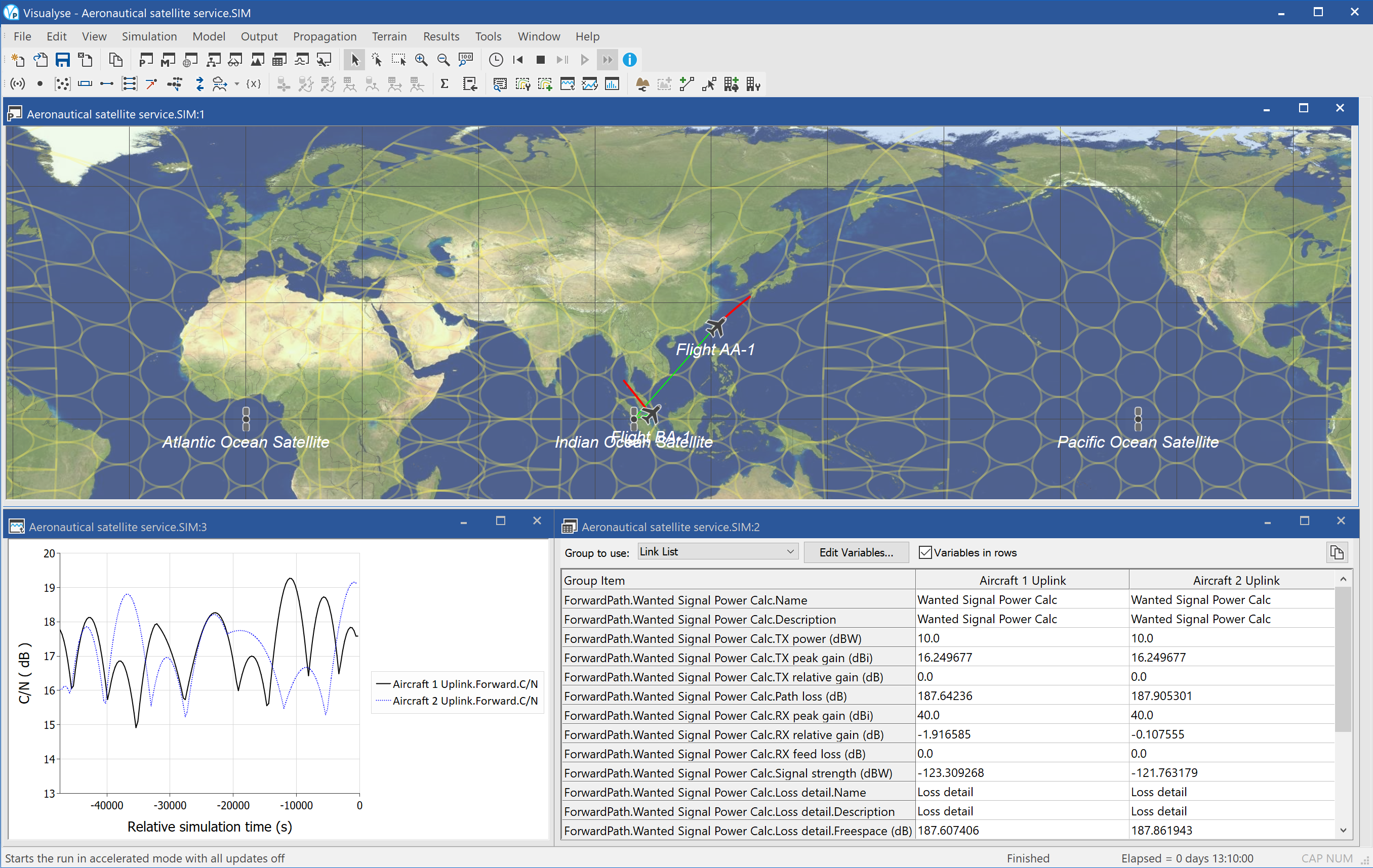
This example shows Visualyse Professional modelling communication between aircraft and GSO satellites.
The simulation uses a dynamic modelling whereby the planes are “flown” across the world from Europe/US to Asia. During the route, they access broadband services via a network of GSO satellites, one for each ocean region.
To provide the high gain needed to close the link, the GSO satellite uses an antenna that generates 89 thin spot beams covering the field of view. As the aircraft moves it must hand-over between these beams.
Visualyse Professional is calculating the C/N of the uplink as the aircraft moves and switches between beam assuming free space path loss and gaseous absorption in ITU-R Rec.P.676.
The figure above shows the simulation with three views open:
- Plate Carrée map view (top) showing the aircraft, the satellites, the satellite spot beams, the links, and the tracks of the aircraft
- Quick graph (bottom left) showing the how the C/N for each link varies with time. As the aircraft moves this plot will follow the peaks and troughs of the currently active beam
- Table view (bottom right) showing the link budget and satellite spot beam used at the present time step.
Aircraft into FS stations
| Action: | Run simulation |
| Modules used: | None |
| Terrain regions: | None |
| Frequency band: | Ku |
| Station types: | Aeronautical, Fixed |
| Propagation models: | Free space, ITU-R Rec.P.530, Diffraction at visible horizon |
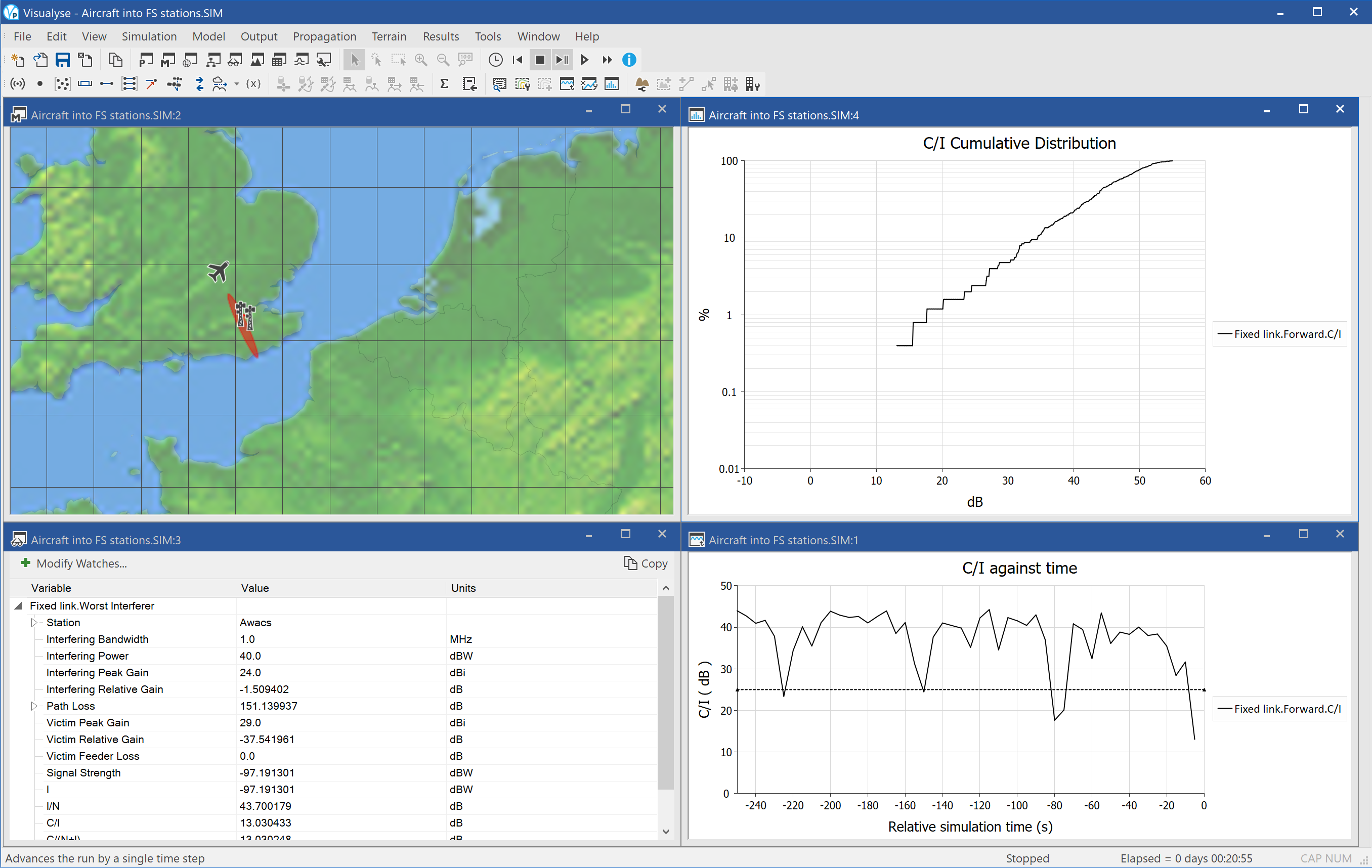
This example shows Visualyse Professional modelling interference from airborne radar into a fixed link at Ku band.
The aircraft is flying across the UK transmitting at high power on a frequency also used by a point to point fixed link. The antenna on the aircraft is rotating round pointing 10 degrees below the horizon and is modelled using ITU-R Rec.F.699 gain pattern. Note the radar antenna spin rate has been reduced to make the example easier to see.
The propagation model for the air to ground is assumed to be free space path loss if line of sight otherwise an additional diffraction term is used.
The fixed link is modelled using free space path loss plus the ITU-R Rec.P.530 rain and fade models which means the wanted signal can vary in time. The fixed link antennas are based upon an ETSI specification style table.
As the aircraft flies and its antenna rotates and the fade varies on the fixed link the C/I changes. When the C/I is below the threshold of C/I = 25 dB the link is assumed to be suffering interference and is shown in red.
The simulation shows the following views open:
- Mercator map view (top left) showing the location of the aircraft, the fixed service stations, the aircraft antenna footprint, and the link coloured as either green (good) or red (bad)
- Watch window (bottom left) showing the interfering link budget from the AWACs to the fixed link
- Statistics graph (top right) showing the cumulative distribution function of the C/I at the fixed link’s receiver
- Quick graph (bottom right) showing how the C/I varies against time together with a line showing the threshold of C/I = 25 dB.
Aircraft with pre-set track across US and interference from FS
| Action: | Run simulation |
| Modules used: | Define Variable |
| Terrain regions: | None |
| Frequency band: | S |
| Station types: | Aeronautical, Fixed |
| Propagation models: | Free space, ITU-R Rec.P.676, Diffraction when beyond line of sight, Aircraft body shielding |
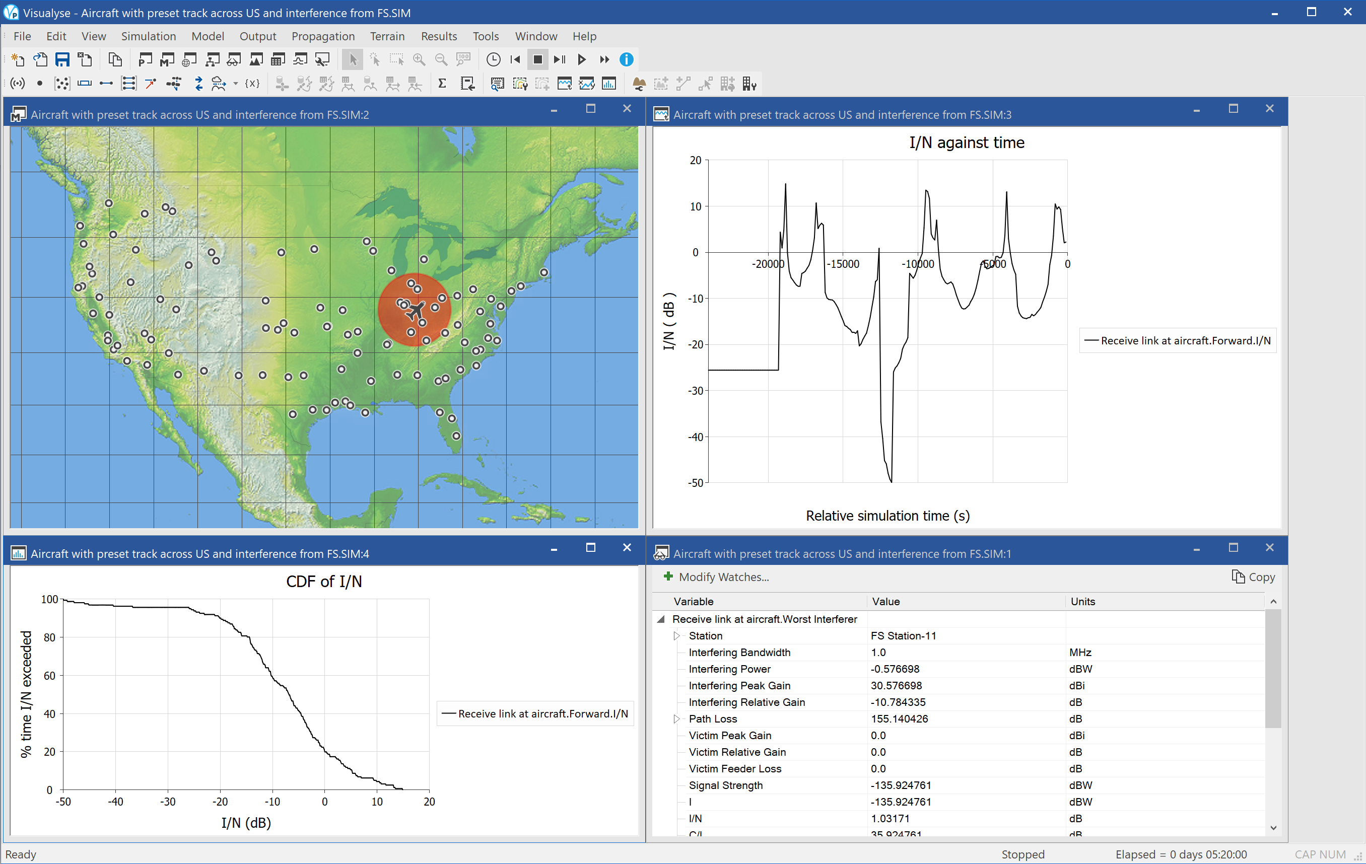
This example shows a scenario whereby a commercial aircraft flies across the US using part of C band (2 GHz) for communication services. This band is also used by a number of point to point fixed links, and therefore there is the potential for interference.
The aircraft is assumed to travel along pre-defined traffic routes: three are modelled:
- Los Angeles to New York
- New York to Seattle
- Seattle to Los Angeles
One hundred fixed service transmitters were deployed across the US, with random antenna azimuth and elevations. Each was assumed to have a single antenna using ITU-R Rec.P.699 as its gain pattern assuming a 2m dish.
The propagation model from the FS to the aircraft included the following four terms:
- Free space path loss
- Diffraction when aircraft is beyond visible line of sight of the fixed station
- Attenuation due to atmospheric gases in ITU-R Rec.P.676
- Shielding loss due to body of aircraft
- The aggregate I/N at the receiver on the aircraft is then calculated from all one hundred of the FS transmitters.
The simulation is shown with four windows open:
- Mercator view (top left) showing the aircraft, its field of view and each of the fixed service transmitters
- Statistics view (bottom left) showing the cumulative distribution function of I/N
- Quick plot (top right) showing how the I/N would vary against time
- Watch window (bottom right) showing the worst single interfering link budget and the aggregate interference
AMT vs. Globalstar
| Action: | Run simulation |
| Modules used: | Define Variable |
| Terrain regions: | None |
| Frequency band: | C |
| Station types: | Non-GSO Satellite, Earth Station, Aeronautical |
| Propagation models: | Free space |
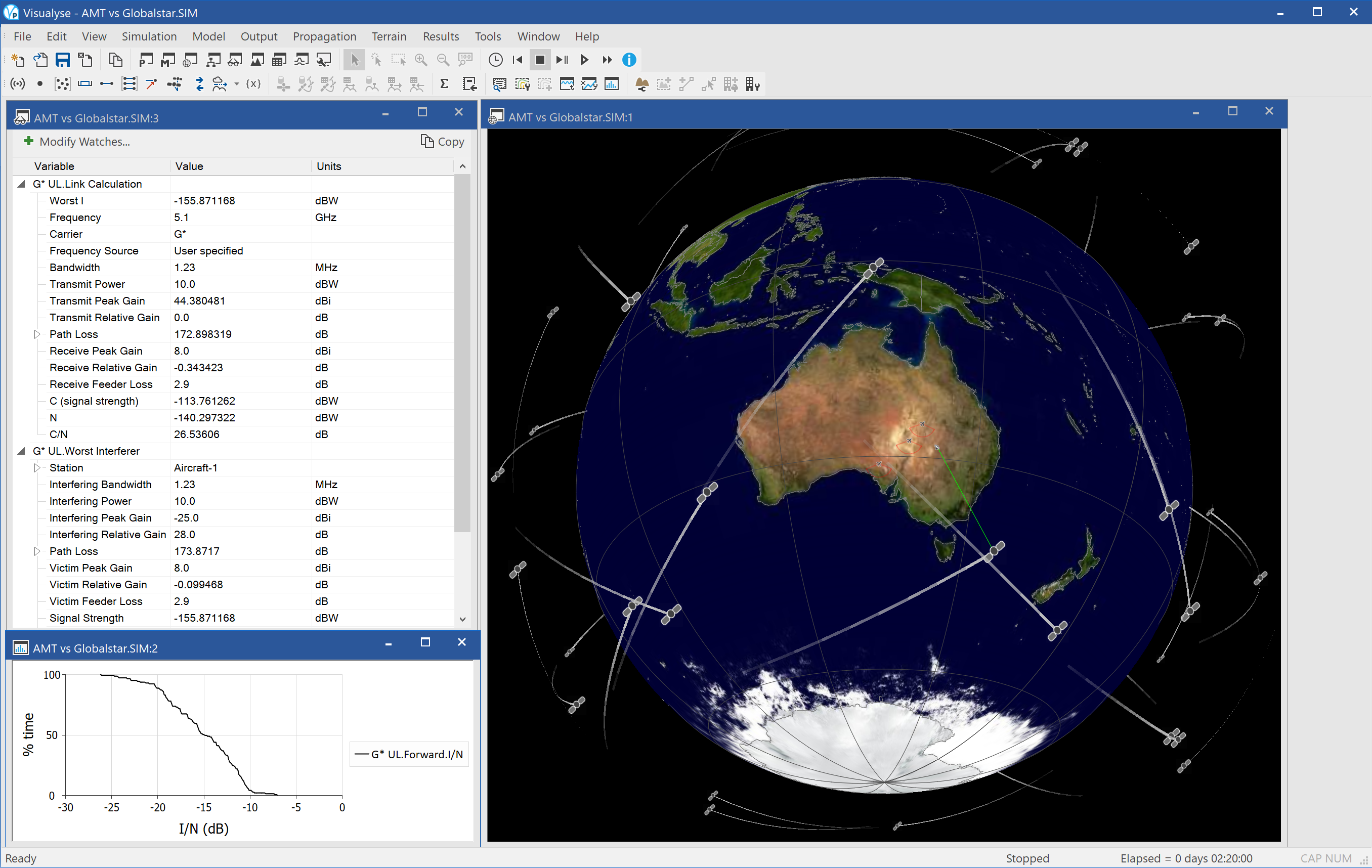
This scenario relates to sharing between aeronautical mobile telemetry (AMT) and non-GSO MSS feeder links at around 5 GHz. In the study cycle leading up to WRC 07 it was Agenda Items 1.5 and 1.6.
The simulation is configured with the victim being the uplink to the Globalstar (G*) network from a gateway in Australia. Co-frequency are a number of aircraft being tested in the desert using the same frequency.
The Define Variable module is being used to specify the location of the aircraft either:
- On a square flight path
- Selected at random using Monte Carlo methods
On each aircraft there are two antennas – one pointing up and one pointing down. The interference is then the aggregate at the satellite receiver of all antennas on all aircraft.
The propagation model for the wanted link from the gateway to the satellites and the interfering link from the aircraft to the satellites is assumed to be simply free space path loss.
In the simulation file, there are three windows open:
- 3D view (right) showing the satellites, their space tracks, the gateway earth station, the link connecting the gateway to the highest elevation satellites, the aircraft and their field of views.
- Watch window (top left) showing the wanted and interfering link budgets
- Statistics window (bottom left) showing the cumulative distribution function of the I/N at the satellite. In this case the highest I/N is predicted to be around -7.5 dB
Modelling air traffic routes
| Action: | Run simulation |
| Modules used: | Define Variable |
| Terrain regions: | None |
| Frequency band: | any |
| Station types: | Aeronautical |
| Propagation models: | n/a |
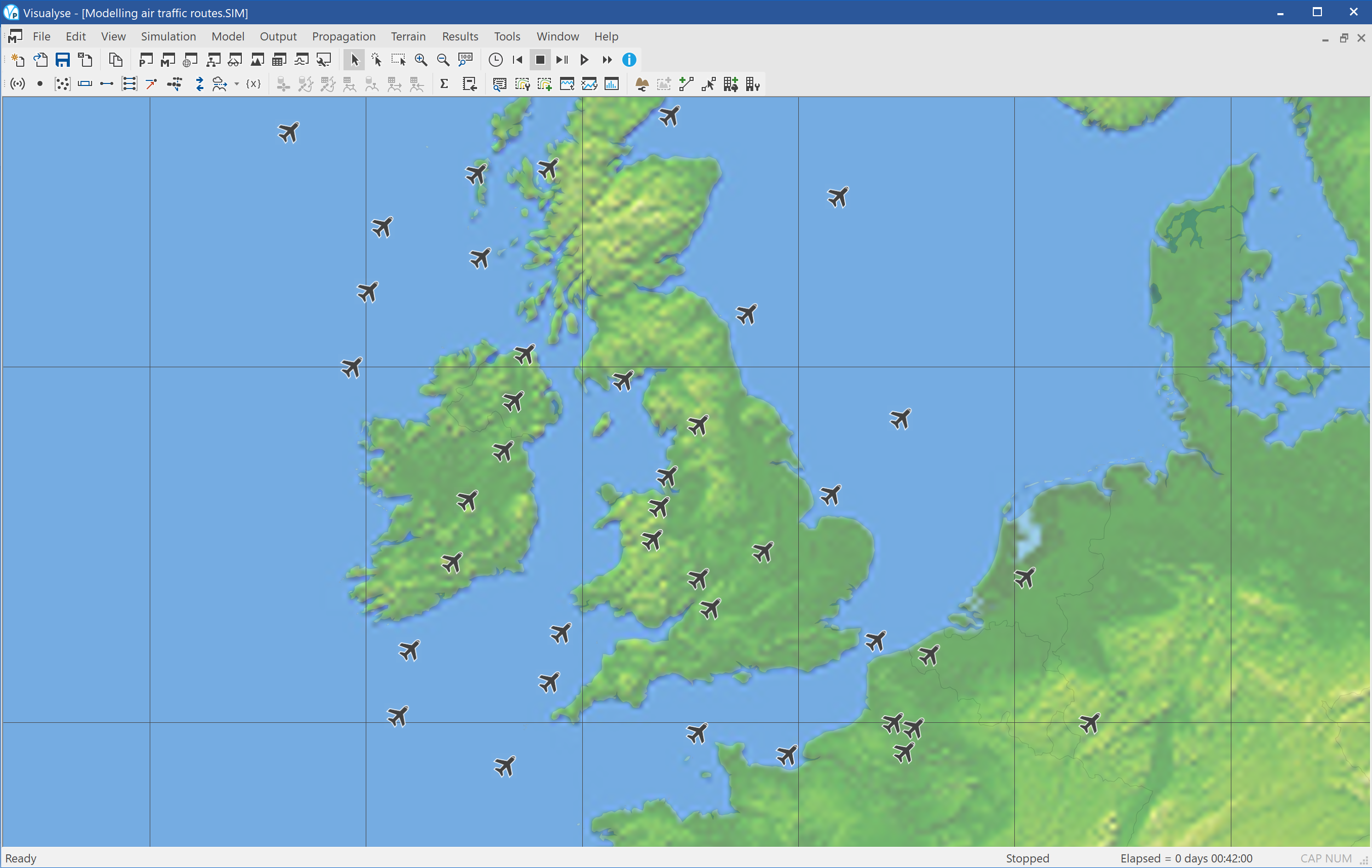
This simulation shows how aircraft traffic routes can be modelled in Visualyse Professional. The simulation shows a number of routes in the vicinity of the UK, some of which are short-haul and some of which are long haul.
A single view is open showing a map of Europe in Mercator projection.