Space Science Service
This section contains the following examples:
- PFD from non-GSO satellite DL
- P-MP FS into EESS (passive)
- Sensor pointing at defined (az, el) angles
PFD from non-GSO satellite DL
| Action: | Run simulation |
| Modules used: | None |
| Terrain regions: | None |
| Frequency band: | X |
| Station types: | Non-GSO Satellite, Earth Station |
| Propagation models: | Free Space |
This example considers the case of a non-GSO satellite being used for remote sensing applications. It is downloading using a directional antenna to an Earth Station in the centre of a large country (India) but there is still the potential to exceed the relevant PFD limits.
These are defined in Article 21 of the Radio Regulations and for the part of X band under consideration, namely around 8 GHz, the limits are:
- -140 dBW/m^2/4 kHz for elevation angles greater than 25°
- Linear interpolation between -140 and -150 dBW/m^2/4 kHz for elevation angles between 5° and 25°
- -150 dBW/m^2/4 kHz for elevation angles less than 5°
The Radio Regulations give each Administration the right to exceed these levels within their own territory. The question is then would these PFD limits be exceeded in adjacent countries?
This simulation shows how Visualyse Professional can help analyse these problems. A set of test points have been defined around the border of a neighbouring country, Pakistan, and the PFD at each test point calculated as the satellite moves along its orbit.
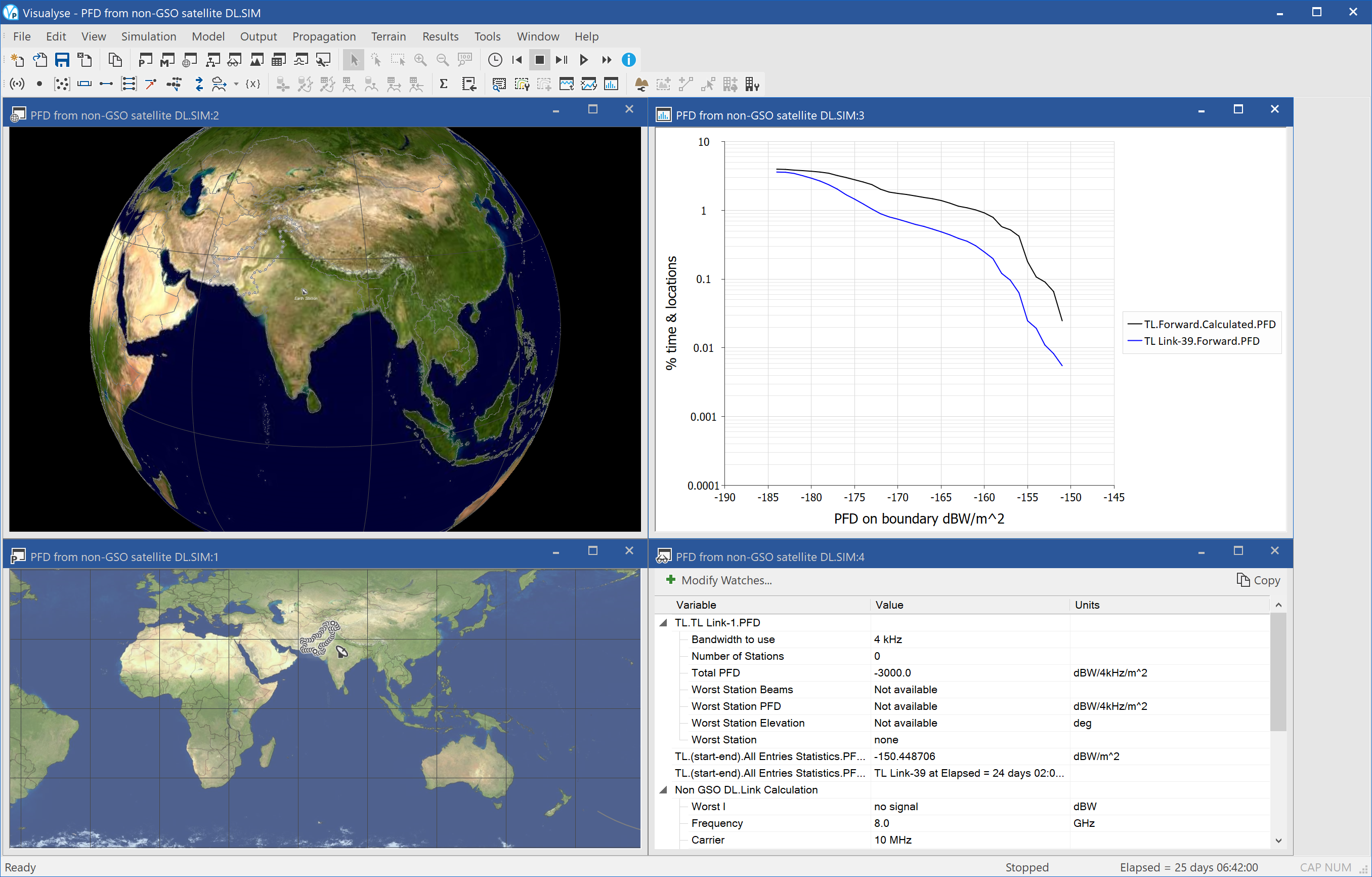
The figure above shows four windows:
- 3D view (top left) showing the non-GSO satellite, its orbit track, the Earth Station, the beam from the non-GSO satellite to Earth Station, and the test points around the adjacent country
- Plate Carrée map view (bottom left), also showing the non-GSO satellite, its orbit track, the Earth Station, the beam from the non-GSO satellite to Earth Station, and the test points around the adjacent country
- Watch window (bottom right) showing the PFD calculation for one of the test points, the worst PFD over all the test points, and the link budget for the X-band downlink
- Statistics graph (top right) showing the cumulative distribution function of the worst PFD at each time step and the CDF of the PFD for one test point (number 39)
Note that the non-GSO satellite only transmits when it can see the Earth Station and the PFD statistics are only updated when the non-GSO satellite is transmitting and can see the test points: hence the statistics are unlikely to be valid for more than 10% of the time. However in this case it can be seen that the PFD limits are met as the PFD never exceeds -150 dBW/m^2/4 kHz.
This simulation can be extended to undertake more advanced analysis which takes account of how the PFD varies with elevation angle.
P-MP FS into EESS (passive)
| Action: | Run simulation |
| Modules used: | Define Variable |
| Terrain regions: | None |
| Frequency band: | Ku |
| Station types: | Non-GSO Satellite, Fixed |
| Propagation models: | Free space path loss, ITU-R Rec.P.676 |
This example shows analysis from large numbers of terrestrial transmitters into a passive space-borne sensor. In this example it involves Ku band point to multi-point (P-MP) fixed service base station interfering with a satellite sensor. There are many other possible examples – including RLANs at 5 GHz into non-GSO MSS feeder links and Ka band SRR into EESS sensors.
In this example 105 P-MP base stations have been deployed across Europe. Their antenna is omni-directional with elevation dependency as in the figure below:
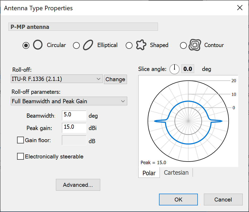
This uses one of the P-MP gain patterns in ITU-R Rec.F.1336. Each one is transmitting at 40 dBm i.e. 10 dBW across a WiMAX channel bandwidth of 10 MHz.
A remote sensing satellite is in orbit overhead, with sensor moving in pre-defined angles using the Define Variable Module. As it flies over Europe is suffers interference at its receiver, measured using the I/N metric.
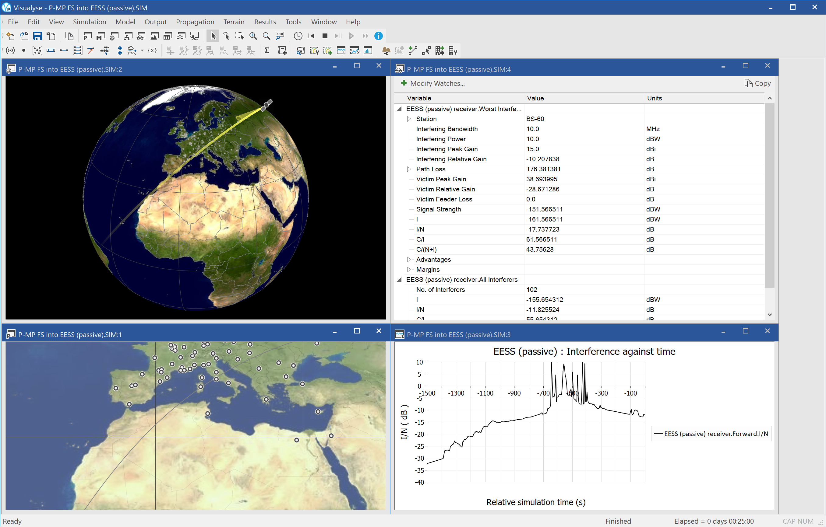
The screen-shot above shows the following windows:
- 3D view (top left): showing the locations of the P-MP base stations, the satellite, its beam, and its space track
- Plate Carrée map (bottom left): showing the locations of the P-MP base stations, the satellite, its beam, and its ground track
- Watch window (top right): showing the link budget for the worst single interfering P-MP base station and the aggregation of all visible interferers
- Quick graph (bottom right): showing how the I/N varies with time as the satellite flies over
It can be seen that in this case the I/N peaks at around 10.8 dB – which could cause significant data loss.
Sensor pointing at defined (az, el) angles
| Action: | Run simulation |
| Modules used: | Define Variable |
| Terrain regions: | None |
| Frequency band: | Any |
| Station types: | Non-GSO Satellite |
| Propagation models: | n/a |
This example shows how the pointing angles of sensors can be defined in a range of different ways in Visualyse Professional. In this example the sensors are on a non-GSO satellite – for example a remote sensing satellite – but they could be on any station type.
There are four satellites each using a different method to point their sensor:
- Fixed pointing: the sensor points with (az, el) = (40°, 0°) for the duration of the simulation
- Swept broom pointing: the sensor scans back and forth between (az, el) angles of (-40°, 0°) and (+40°, 0°) at a rate of 1° per second
- Rotating: the sensor scans round around through-out 360° at a fixed elevation angle – in this case -55° – at a scan rate of 1° per second. Note that the scan platform was rotated through -90° of pitch using the Euler angles under “Advanced” so the rotation is around the required axis
- Pre-defined: the Define Variable Module was used to vary the pointing to specific locations at pre-defined times with interpolation between angles defined in the look-up tables
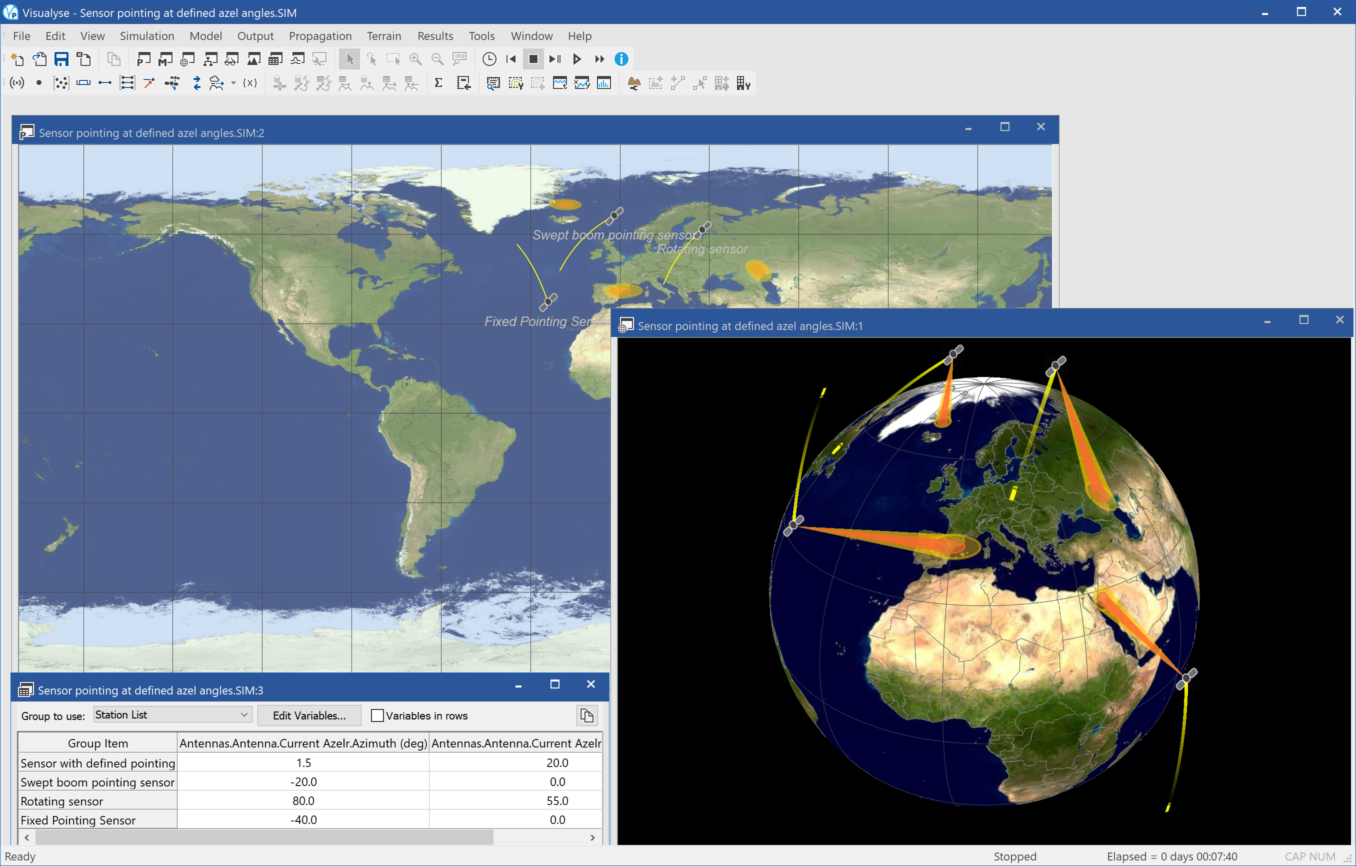
The simulation has been configured with three windows open:
- Plate Carrée map view (top) showing the location of the satellites, their beam footprints (-3 dB and -10 dB contours), and the ground tracks
- 3D view (right) showing the location of the satellites, their beam footprints (-3 dB and -10 dB contours), and the space tracks
- Table view (bottom left) showing the (az, el) angles of the sensors for each of the satellites.