Coordination Systems

This section defines the coordinate systems used for each type of station and within antennas and beams.

• ECI Vectors
• Terrestrial Stations
• Satellite Orbits
• Station Coordinate Systems
• Station, Antenna and Beam Coordinate Systems
• Slice Angle

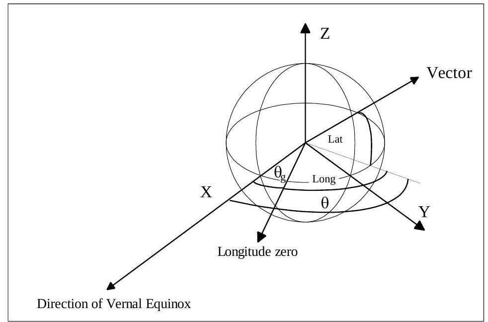
ECI Vectors

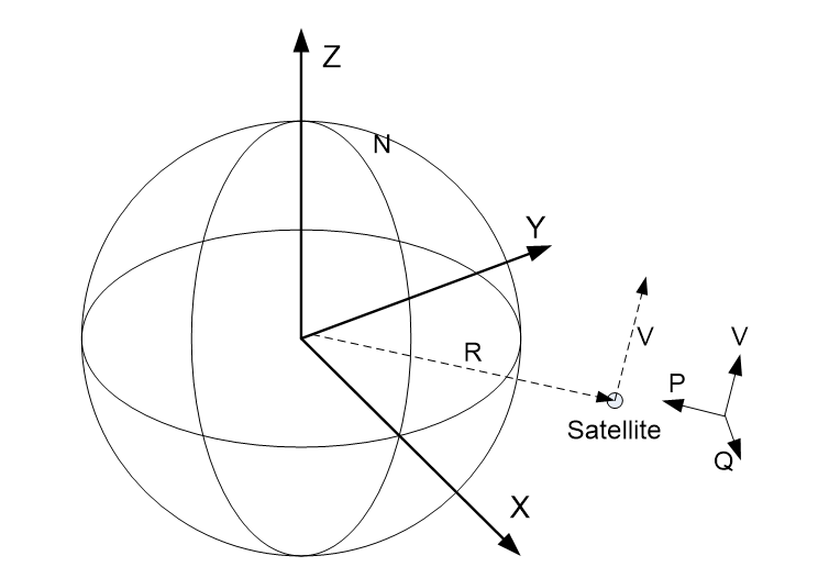
All stations in Visualyse Professional are located in Earth Centred Inertial (ECI) coordinate system using position and velocity vectors of the form:

$$r=\left(\begin{array}{l}x\\ y\\ z\end{array}\right)$$

The co-ordinate system is defined as follows:

X axis: aligned with the vernal equinox as described further below

Z axis: aligned with the North Pole

Y axis: at right angles to the X and Z axes, using right handed co-ordinate system

The X axis of the ECI system is oriented in relation to the earth using the first point of Aries at the following epoch:

At: 00:00 hours on the 1st January 1970

$${\theta }_{g_0}=100^{\circ }229421$$

This is shown in the figure below:

The frame of reference of the earth rotates at the following rate:

$${\theta }_g={\theta }_{g_0}+\omega t$$

Where:

$\omega$ is the angular rotation rate of earth in radians / second

$\mathrm{t}$ is time in seconds since reference time

Terrestrial Stations

Stations on the surface of the Earth are defined via their (latitude, longitude, height) which is converted into an ECl vector using:

$$\underline{r}=R\left(\begin{array}{c}\cos (lat)\cos \left({\theta }_g\right)\\ \cos (\text{ lat })\sin \left({\theta }_g\right)\\ \sin (\text{ lat })\end{array}\right)$$

Where:

$R=$ Radius of the Earth $\left(R_e\right)+$ height of station above smooth Earth (h)

Lat $=$ Latitude of the station

${\theta }_g=$ the conversion of the longitude in the rotating Earth frame to angle with respect to the $X$ axis.

Stations with non-zero speed will have their (latitude, longitude, heights) updated assuming they take great circle paths over a spherical Earth.

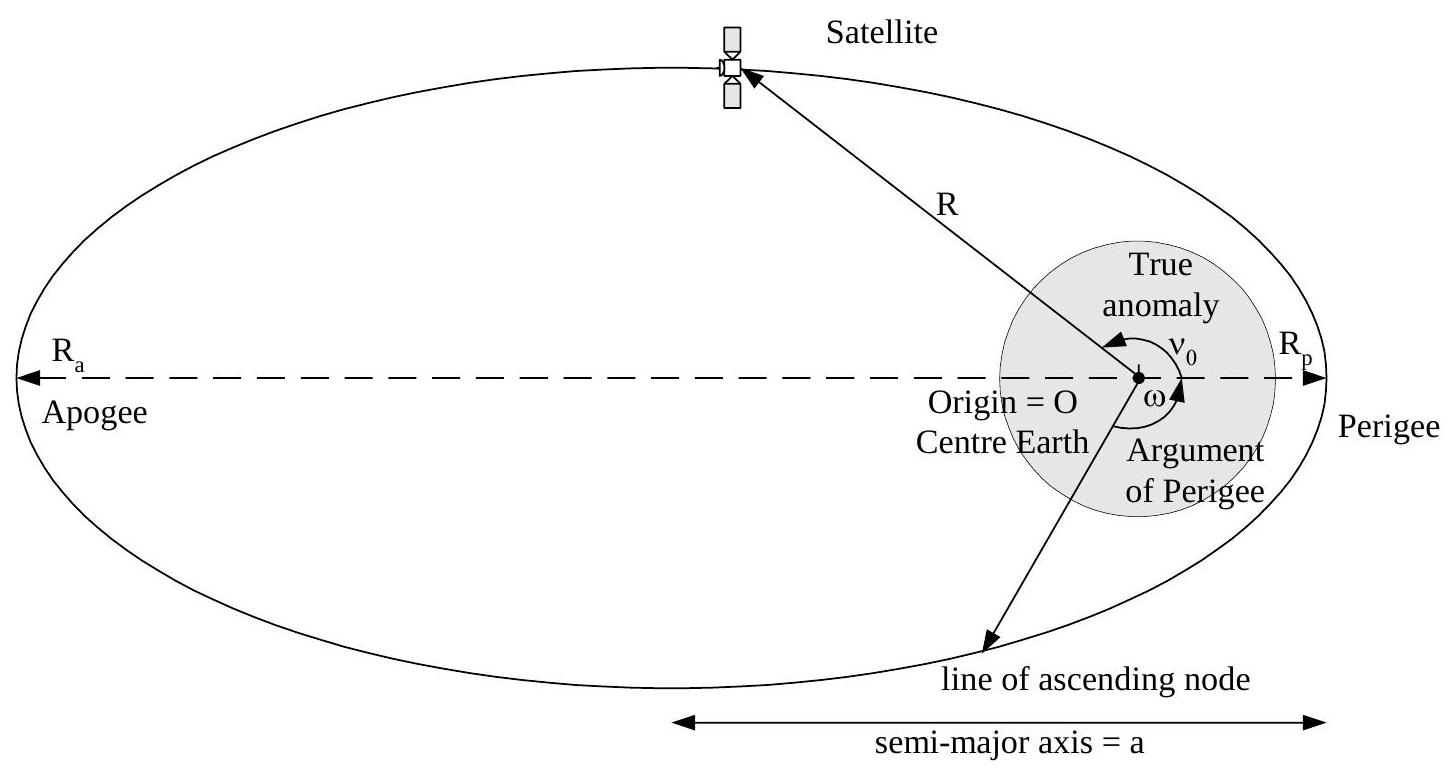
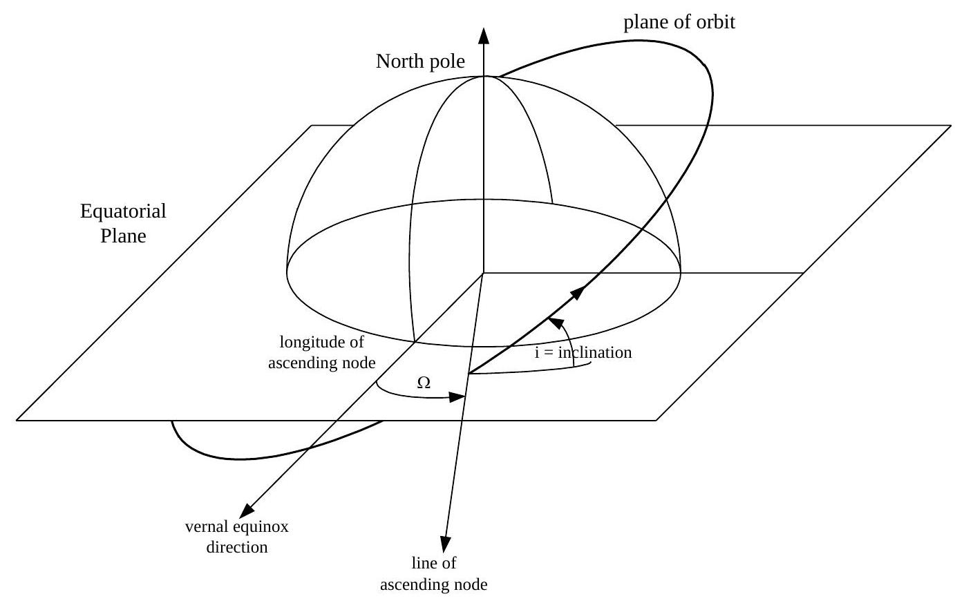
Satellite Orbits

• Orbit Parameters
• Orbit Models
• Orbit Conversions

Orbit Parameters

Within Visualyse Professional a standardised set of orbital elements are used, namely:

These parameters are shown in the figures below.

Orbit Models

Two orbit models are including in Visualyse Professional:

• Point mass
• Point mass plus $J2$ term

The $\mathrm{J}2$ orbit model to update a non-GSO satellite at time $\Delta \mathrm{t}$ is calculated from the orbit elements as follows:

$$\begin{array}{rl}& \mathrm{a}={\mathrm{a}}_0\\ & \mathrm{e}={\mathrm{e}}_0\\ & \mathrm{i}={\mathrm{i}}_0\\ & \omega ={\omega }_0+{\omega }_r\Delta t\\ & \Omega ={\Omega }_0+{\Omega }_r\Delta t\\ & M=M_0+\left(\bar{n}+n_{\text{user }}\right)\Delta t\end{array}$$

Where:

${\omega }_0:$ perigee argument at an initial moment

${\Omega }_0:$ ascending node longitude at an initial moment

${\mathrm{M}}_0:$ mean anomaly at initial moment

${\mathrm{n}}_{\text{user: }}$ additional, user entered, precession (defaults to zero)

And:

${\omega }_r:$ perigee argument precession rate

${\Omega }_r:$ ascending node longitude precession rate

$\bar{n}:$ rate of change of mean anomaly

These are calculated from the following:

$$\begin{array}{rl}& {\omega }_r=\frac{3}{2}\frac{J_2{R}_e^2}{p^2}\bar{n}\left(2-\frac{5}{2}{\sin }^2(i)\right)\\ & {\Omega }_r=-\frac{3}{2}\frac{J_2{R}_e^2}{p^2}\bar{n}\cos (i)\\ & \bar{n}=n_0\left(1+\frac{3}{2}\frac{J_2{R}_e^2}{p^2}\left(1-\frac{3}{2}{\sin }^2(i)\right){\left(1-e^2\right)}^{1/2}\right)\end{array}$$

where:

$$\begin{array}{rl}& p=a\left(1-e^2\right)\\ & J_2=1.083e-3\\ & n_0=\sqrt{\frac{\mu }{a^3}}\end{array}$$

Orbit Conversions

Some orbits are defined using other parameters, such as apogee / perigee height or radii. These can be converted into the standard set above using the following equations.

Elliptical orbit shape

The apogee / perigee heights / radius's can be converted using:

Apogee conversion: $R_a=R_e+h_a$

Perigee conversion: $R_p=R_e+h_p$

${\mathrm{R}}_{\mathrm{e}}$ is the Earth's radius of $6378.1\mathrm{km}$.

Then the semi major axis and eccentricity are:

$$\begin{array}{rl}& R_a=a(1+e)\\ & R_p=a(1-e)\end{array}$$

So:

$$\begin{array}{rl}& a=\left(R_a+R_p\right)/2\\ & e=\left(R_a-R_p\right)/\left(R_a+R_p\right)\end{array}$$

Anomaly Angle

There are a number of ways of defining where the satellite is in the orbit plane with respect to the perigee, including

$$\begin{array}{rl}& v=\text{ true anomaly }\\ & E=\text{ eccentric anomaly }\\ & M=\text{ mean anomaly }\end{array}$$

These are related using:

$$\begin{array}{rl}& \cos E=\frac{e+\cos v}{1+e\cos v}\\ & \cos v=\frac{e-\cos E}{e\cos E-1}\\ & M=E-e\sin E\end{array}$$

The last equation can be used together with iteration to calculate $E$ from $M$.

Elapsed time is related to $M$ using:

$$M=n\Delta T$$

where $n$ is the mean motion:

$$n=\sqrt{\frac{\mu }{a^3}}$$

where $\mu =3.986012\mathrm{e}5{\mathrm{km}}^{\wedge }3/{\mathrm{s}}^{\wedge }2$ is the gravitational constant

Anomaly Angle

There are a number of ways of defining where the satellite is in the orbit plane with respect to the perigee, including

$$\begin{array}{rl}& v=\text{ true anomaly }\\ & E=\text{ eccentric anomaly }\end{array}$$

$M=$ mean anomaly

These are related using:

$$\begin{array}{rl}& \cos E=\frac{e+\cos v}{1+e\cos v}\\ & \cos v=\frac{e-\cos E}{e\cos E-1}\\ & M=E-e\sin E\end{array}$$

The last equation can be used together with iteration to calculate $E$ from $M$.

Elapsed time is related to $M$ using:

$$M=n\Delta T$$

where $n$ is the mean motion:

$$n=\sqrt{\frac{\mu }{a^3}}$$

where $\mu =3.986012\mathrm{e}5{\mathrm{km}}^{\wedge }3/{\mathrm{s}}^{\wedge }2$ is the gravitational constant

Station Coordinate Systems

The coordinate system used by the station defines how the antennas are pointed and varies between station types.

• Calculation of Azimuth and Elevation
• Fixed Stations
• Non Geostationary Satellites
• Geostationary Satellites
• Moving Stations

Calculation of Azimuth and Elevation

For each station type an intermediate local set of orthogonal vectors, (X’, Y’, Z’) are generated. From these the azimuth and elevation are calculated as follows:

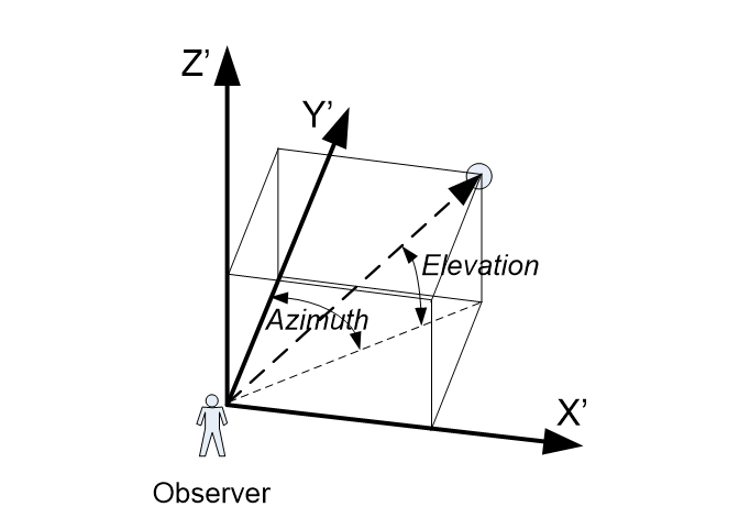
To define the coordinate system for each station type it is therefore necessary to define the ( $X^{\prime },Y^{\prime },Z^{\prime })$ vectors in each case.

An alternative way of considering it is that for an observer, the azimuth is the angle in the horizontal plane with the line directly ahead, with the right hand being positive, whilst the elevation is the angle in the vertical plane compared to the horizon, with up being positive.

Fixed Stations

For stations at fixed locations, whether Earth, terrestrial, mobile, maritime or aeronautical stations, the azimuth and elevations are derived using the north, east and zenith vectors as shown in the figure below:

Figure Earth / Terrestrial station co-ordinate system

These are mapped onto the generic local vectors as follows:

X’ = E

Y’ = N

Z’ = Z

The result is the traditional alignment of:

• Azimuth = angle in the horizontal plane from due North increasing in a clockwise direction, defined within the range (-180 to +180)
• Elevation = angle above the horizontal plane

Non Geostationary Satellites

For satellites the coordinate system is based upon the line to the centre of the Earth (i.e. towards the sub-satellite point) and the velocity vector, so that for circular orbits:

X’ = Q = vector at right angles to velocity and position vectors

Y’ = P = -R

Z’ = V

The P and Q vectors are shown in the figure below.

Another way of looking at it is to consider the view from the satellite looking down at the sub-satellite point, head pointing in the direction of the velocity vector – the “superhero” position. In this case as in the figure below:

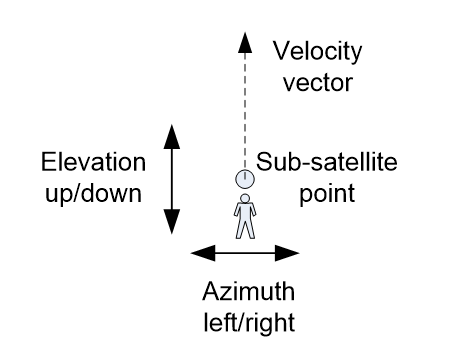
• Azimuth = to left and right of the sub-satellite point, where right is positive
• Elevation = up and down, where up is positive

This coordinate system assumes that the radius vector and velocity vector are at right angles which will only be the case for circular orbits. For elliptical orbits it is necessary to select which vector of (R, V) the coordinate system will align with.

Geostationary Satellites

For satellites the coordinate system is based upon the line to the centre of the Earth (i.e. towards the sub-satellite point), the north vector, and the velocity vector, so that:

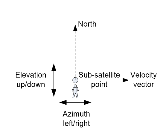
Figure 3: Coordinate System for Geostationary Satellites

In formal terms, for a GSO satellite:

X’ = V

Y’ = -R

Z’ = N

Moving Stations

Moving stations can use either of the coordinate systems describe above:

• North based, as for terrestrial stations
• Velocity based, as for non-GSO satellites.

Additional coordinate frames can be created by utilising the orientation (or Euler) angles (pitch, roll, yaw) which define how the antenna platform is located with respect to the station coordination scheme.

For example consider an aircraft, when the orientation is velocity based, where the following Euler angles have been set:

Pitch = 90º

Roll = 0º

Yaw = 0º

This will rotate the az/el = (0, 0) line from the line from the station to the centre of the Earth to the direction of motion. Having done this the azimuth angle is similar to yaw while elevation angle similar to pitch, as in the figure below using a ship as an example:

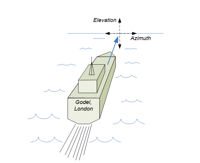
A similar coordinate system can be used for aircraft.

Note that if the aircraft is pitching up or down the velocity vector will not be at right angles to the position vector. Hence the coordinate frame will have to choose which to align with.

To create a coordinate system in which the reference az/el = (0, 0) remains the nose of the aircraft even when pitching up or down the following settings should be used:

Coordinate System:

Velocity based = true

Align with velocity vector = true

Pitch = 90º

Roll = 0º

Yaw = 0º

Station, Antenna and Beam Coordinate Systems

A station can contain multiple antennas which can contain multiple beams. Each can have its own pointing angles – so for example there can be:

• Pointing angles of antenna with respect to station’s coordinate system (these are the azimuth, elevation of the antenna in the station dialog)
• Pointing angles of beam with respect to antenna’s coordinate system (these are the azimuth, elevation of the beam in the antenna dialog)

In addition there can also be:

• Pointing angles of antenna platform with respect to station (these are the orientation angles on the station dialog’s advanced tab)

These angles are combined together in the following order from inertial ECI vectors:

• From ECI to (azimuth, elevation) in station coordinate system using definition of (X’, Y’, Z’) in previous section
• From station coordinate (azimuth, elevation) to antenna platform (azimuth, elevation) using orientation angles (yaw, pitch, roll)
• From antenna platform (azimuth, elevation) to a specific antenna’s (azimuth, elevation) using the antenna’s az/el pointing angles
• From an antenna’s (azimuth, elevation) to a beam’s (azimuth, elevation) using the beam’s az/el pointing angles

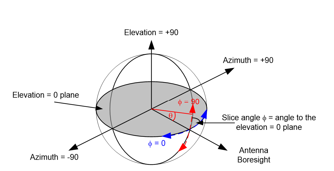
Slice Angle

This section describes the definition of the slice angle which is used within Visualyse Professional to display gain patterns.

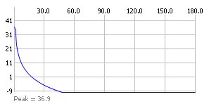
For many antennas, such as those using parabolic reflectors, the gain pattern is symmetric around the boresight. The gain pattern can therefore be displayed in a graph as gain vs offaxis angle – for example the pattern below is Recommendation ITU-R Rec. S.465 for a 2.4m dish at 3.6 GHz:

Other antennas do not have this symmetry: for example the patterns of a base station antenna are likely to vary in both azimuth and elevation, and hence are described as 3D patterns.

For these antennas the gain pattern taken in the azimuth and elevation directions are likely to be different, and we call these different directions “slices”. The slices are taken in planes that intersect the boresight line (see figure at top).

The orientation of the slice is defined by the slice angle or , which is the angle of the slice plane to the elevation = 0 plane. Hence the = 0 slice is the gain pattern in the azimuth plane while the = 90 slice is the gain pattern in the elevation plane.

Rather than showing offaxis angle along the X axis of the gain plot, the slice instead shows the angle from the boresight line, shown in the figure above as .

Any slice angle can be selected from 0 to 180 and it will define a plane and hence create a separate gain pattern. As all slices intersect the boresight line all will start with the = 0 point which is the boresight, usually, but not always, defined as the point in the 3D gain pattern with highest gain value.

For example the figures below show two slices from the same 3D gain pattern and hence start with = 0 where the gain = 18 dBi.

Slice angle = 0 (azimuth plane)	Slice angle = 90 (elevation plane)

Note that azimuth and elevation in this figure are relative to the gain pattern’s boresight and there could be a variety of orientation angles including:

• Beam within the Antenna Type
• Antenna with respect to the Antenna Platform
• Antenna Platform with respect to the Station

Note also there are a variety of Station orientations as described in the previous sections.