Others
This section contains the following examples:
HAPS with FS and FSS
| Action: | None |
| Modules used: | None |
| Terrain regions: | None |
| Frequency band: | C |
| Station types: | GSO Satellite, Earth Station, Fixed Station, Aeronautical |
| Propagation models: | Free space, ITU-R Rec.P.676 |
This example shows sharing between a High-Altitude Platform Station (HAPS) and terrestrial point to point Fixed Service station and satellite Earth Stations.
The HAPS network has been configured with two sets of antennas:
- Multiple beam service link antenna
- Spot beam used as feeder to gateway station
This example considers use of some of the upper parts of C band for the feeder link. It is assumed that this is shared with terrestrial receivers, which are modelled using ITU-R Rec.F.699 as the gain pattern and a range of locations (latitude, longitude) and pointing angles (azimuth, elevation). These could either come from real assignment data read in using one of:
- Interface to the ITU-R’s database of terrestrial assignments (IFIC)
- FS import tool using spreadsheet or CSV format data
There are also a number of GSO satellite earth stations which could suffer interference from the HAPS.
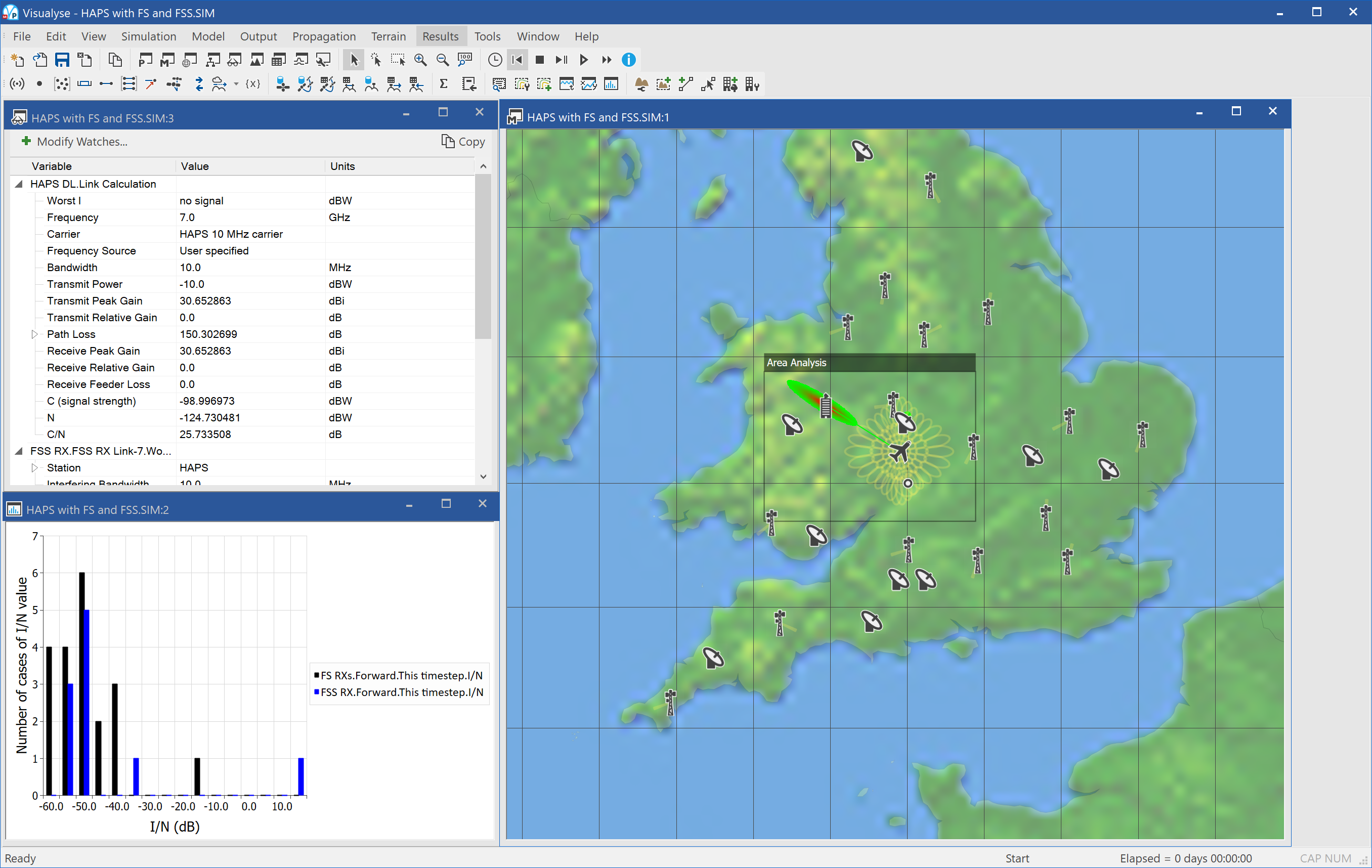
The simulation above shows the following windows:
- Mercator view (right) showing the HAPS aeronautical station, its service links beams, its feeder link, the HAPS gateway, the various earth stations, the fixed link stations and their azimuths
- Watch window (top left) showing the link budget for the HAPS downlink and also the interference calculation from the HAPS into one of the Earth Stations (the worst case one with I/N around 17 dB)
- Statistics graph (bottom left) showing a histogram of the I/N across the various fixed and fixed satellite service receivers. It can be seen that the worst I/N is around 17 dB
The view also shows an Area Analysis of locations where putting an Earth Station that could make it susceptible to interference. There are two vulnerable geometries:
- Around the HAPS gateway
- Cases where the HAPS would be directly in line between the Earth Station and its satellite.
Smart Antennas
| Action: | Run simulation |
| Modules used: | Define Variable |
| Terrain regions: | None |
| Frequency band: | S |
| Station types: | Mobile, Fixed |
| Propagation models: | Hata / COST231 |
This simulation shows an example of the analysis of the impact of using smart antennas. These can be used, for example, by base stations of mobile networks to improve performance. Rather than having fixed pointing and cover a fixed area – for example 90° of azimuth – a smart antenna creates a focussed beam of energy towards the wanted direction.
In this simulation we have two base stations:
- Using conventional 120° sectors, with downtilt of 2° and peak gain 15 dBi
- Using a number (up to 25) narrow spot beams that point at a mobile as required with peak gain 30 dBi
Within the cell of each base station there located at random two mobile stations, and a link is set up using 3G/WCDMA parameters to close the link for a C/N of around 12.5 dB using power control to determine an appropriate transmit power.
Within this scenario two issues are being addressed:
- Which case would create the highest interference towards other receivers co-frequency?
- Which case would provide the least intra-system interference and hence could provide the highest capacity?
This is analysed by running a Monte Carlo style analysis and producing statistics of I/N at a victim receiver or C/(N+I) for each mobile link assuming the other mobile link also causes interference. It is assumed the intra-system interference path can use orthogonal coding to reduce interference by 10 dB.
Both the wanted and interfering paths are assumed to use the Hata / COST 231 propagation models and operate at a frequency of 2 GHz.
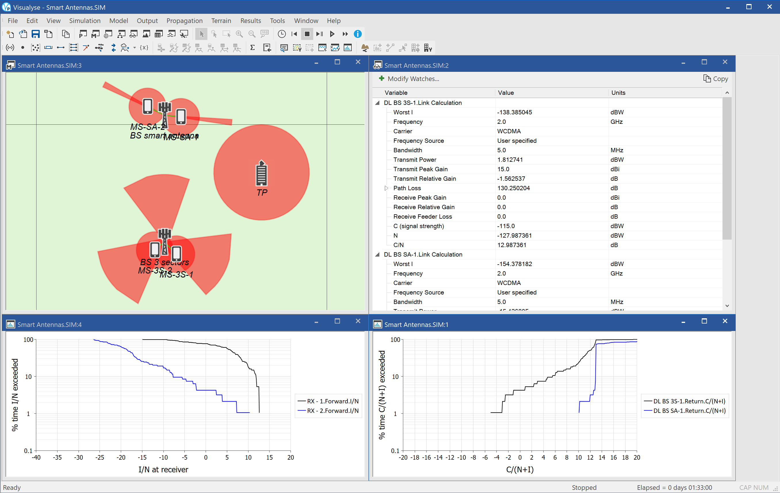
In the screen shot above there are four windows open:
- Mercator map view (top left) showing the locations of the two base stations, the mobiles they are services, their beams, and the test point.
- Statistics graph (bottom left) showing the cumulative distribution function of I/N from each of the two base stations into the receive test point. It can be seen that for all percentages of time the smart antenna base station causes lower levels of interference
- Statistics graph (bottom right) showing the cumulative distribution function of the C/(N+I) for one mobiles for each of the base station taking into account interference from the other within the cell.
- Watch window (top right) showing the wanted link budget calculation for a mobile from the 3 sector and smart antenna systems. The effect of power control on the variation in transmit power can be clearly seen.
Traffic and Exclusion Zone
| Action: | Run simulation |
| Modules used: | Define Variable, Traffic |
| Terrain regions: | None |
| Frequency band: | UHF |
| Station types: | Mobile, Radio astronomy |
| Propagation models: | Hata / COST231 |
This example demonstrates how the Traffic module can be used to model more accurately the behaviour of a mobile network.
A mobile operator wants to deploy at base station in UHF band that would receive uplinks from mobile users in a channel adjacent to that used by the radio astronomy service (RAS). This service has very stringent protection requirements: Recommendation ITU-R RA.769 suggests a threshold of -202 dBW/MHz at the receiver for no more than 2% of time.
One way to protect the radio astronomy service is to employ an exclusion zone, and the mobile operator is suggesting one with radius 5 km would be sufficient. The question is how to test that assumption.
Interference from the uplink can be very variable due the randomisation of the number of active users and their location within the cell. In Visualyse Professional this can be modelled using the Define Variable and the Traffic Module, which can also be used to define an Exclusion Zone.
In this case a traffic object is defined such that a mobile user is active for 25% of the time and never when within 5 km of the RAS site. A variable definition is used to randomise the position of 12 users within a hexagonal cell.
We have assumed the base station at the centre of the cell and is located just outside the exclusion zone, being 6 km away. Power control is used on the uplink and the COST 231 / Hata propagation model used for both wanted and interfering paths.
The RAS is assumed to be operating in UHF channel 38, while the mobiles are in channel 37, so this is an adjacent band analysis. A fixed attenuation of 40 dB is assumed between the 5 MHz WCMDA carrier and a 1 MHz reference receiver bandwidth.
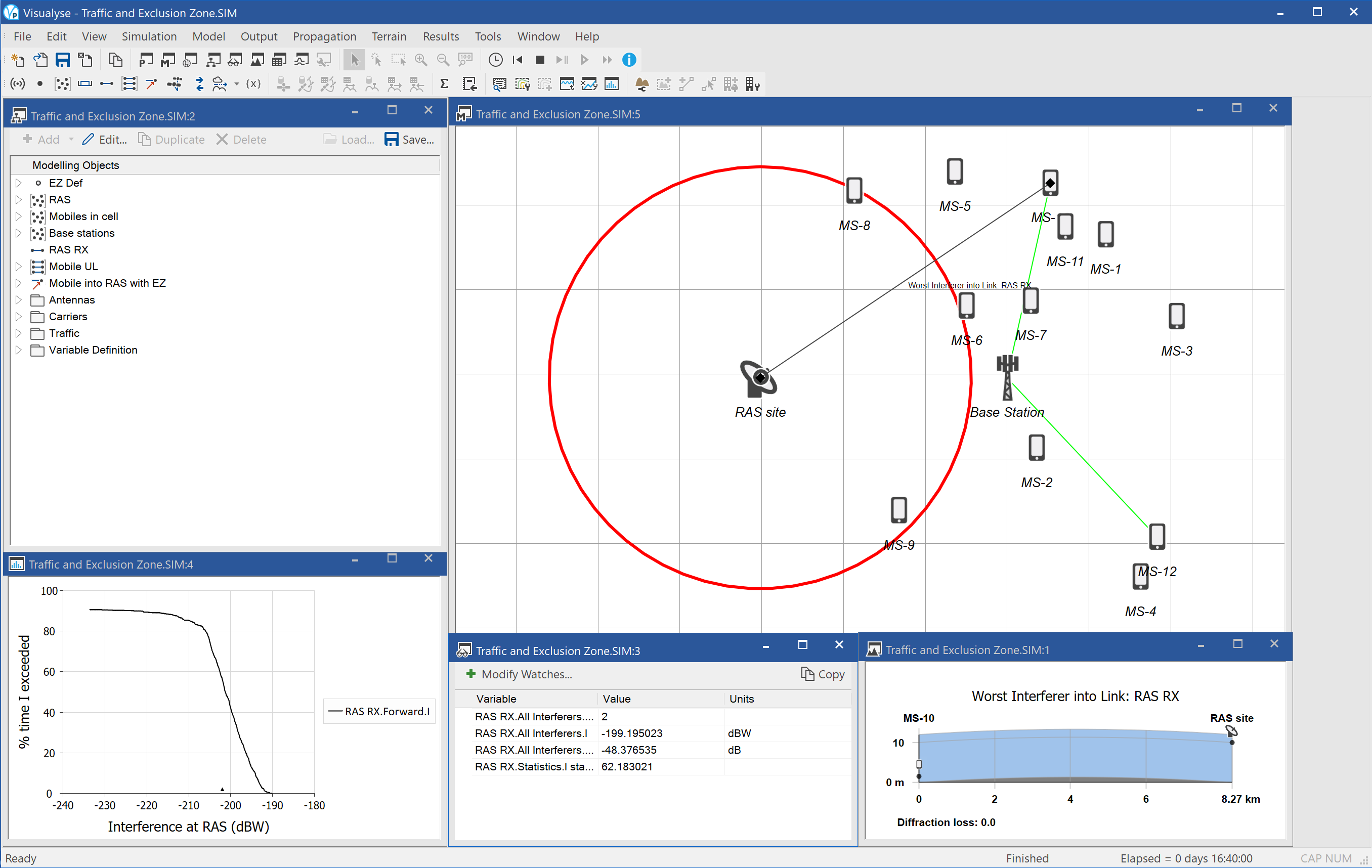
In the screen shot above there are five windows open:
- Model view (top left) showing the various simulation objects in a “file explorer” like display
- Mercator map view (top right) showing the locations of the radio astronomy site, the base station, the mobiles, the active links, and the exclusion zone. Grid lines are every 2 km
- Statistics graph (bottom left) showing the cumulative distribution function (CDF) of interference at the radio astronomy site, with the threshold from ITU-R Rec.RA.769 as a marker. Note how the CDF never reaches 100% as there are times when no mobiles outside the exclusion zones are active
- Watch window (bottom centre) showing the number of interfering entries, the total interference, the I/N at the RAS site, and the percentage of time interference would occur
- Path profile window (bottom right) showing path from the radio astronomy site to the worst single interferer
If you run the simulation you will see the interference exceeds the radio astronomy threshold by around 10 dB and so further mitigation would be required. One simple additional step would be to consider the effect of terrain and clutter.
Note also how the number of interferers changes due to variation in number of active users and whether they are within the exclusion zone or not.
Wi-Fi and ENG
| Action: | None |
| Modules used: | None |
| Terrain regions: | None |
| Frequency band: | S |
| Station types: | Fixed, Mobile |
| Propagation models: | ITU-R P.1791 |
There are a number of bands that are or could be used for Electronic News Gathering (ENG). This example considers one such, use of the licence exempt 2.4 GHz band for ENG.
This is also widely used for wireless access networks using the 802.11 standard, Wi-Fi. The question is then what is the implication of widespread use of the 2.4 GHz band by ENG transmitters.
The scenario considers two Wi-Fi networks, with central node and remote user. The coverage is predicted using a dual slope propagation model based upon ITU-R Rec.P.1791. The simulation considers the downlink direction: it would also be necessary to consider the uplink in more detailed analysis.
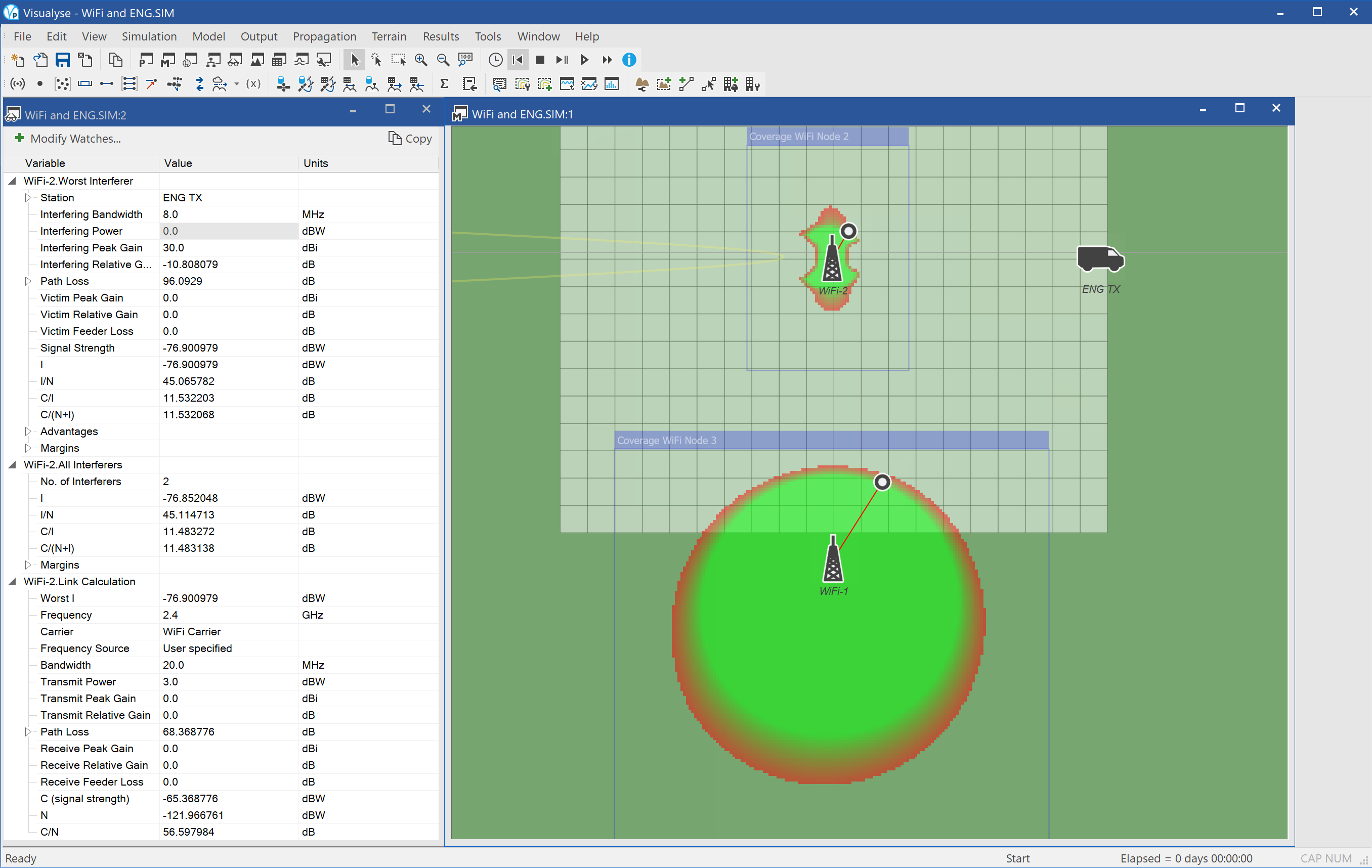
An ENG is modelled as transmitting pointing directly at one of the Wi-Fi nodes, and the impact on coverage modelled taking into account this source of interference. The interference between the Wi-Fi networks is also included. It can be seen that the coverage of the Wi-Fi network is severely reduced by the impact of the ENG, while there is only minor reduction in coverage due to one Wi-Fi node on another1.
The figure above shows two windows open:
- Mercator view (right) showing locations of the Wi-Fi nodes, a test user, the ENG transmitter, and the coverage of each wireless network in the presence of interference. To give an idea on scale, the grid lines are spaced every 10 m.
- Watch window (left) showing link budgets of the wanted and interfering signals of the most effected Wi-Fi user.
-
Note that as 802.11 uses carrier detection to avoid collisions, there is usually time sharing of the radio spectrum between nearby Wi-Fi networks. ↩