Define Variable Module
Introduction
The Define Variable Module allows you to vary the value of any input parameter of any object during a simulation run. The value can be randomised, taken from a sequence or offset from another object attribute. In addition there are tools to Monte Carlo satellites within a non-GSO constellation and mobile stations within a cell.
Under normal circumstances the value of an object attribute is either fixed for the duration of a run or it is changed internally by the simulation. The Define Variable Module gives you the ability to change or control an attribute’s value as a run progresses.
Within Visualyse Professional this is done by a “Variable Definition”, of which there are six types:
- Monte Carlo: a simulation variable is set by randomly sampling values from a number of distributions including Rayleigh, normal, and log normal
- Offset: a simulation variable is set based upon another simulation variable’s value offset by a fixed amount or ratio
- Event table: the variable is set at each time step using interpolation between points of a table of (value, time)
- Sequence: the variables value for each time step is set explicitly
- Monte Carlo Constellation: the position of all the satellites within a non-GSO constellation are randomised while maintaining their relative positions
- Monte Carlo Mobiles: the positions of mobile stations is randomised within a cell around a base station that can be a circle, square or hexagon
Managing Variable Definitions
Variable Definition objects are part of the simulation, stored in the .sim file, and managed via a list where they can be created, deleted, duplicated, and modified.
The Variable Definition list can be accessed via the “Model” menu option “Variable Definition” or by the toolbar icon: ![]()
Selecting either of these will open the Variable Definition list, as shown below.
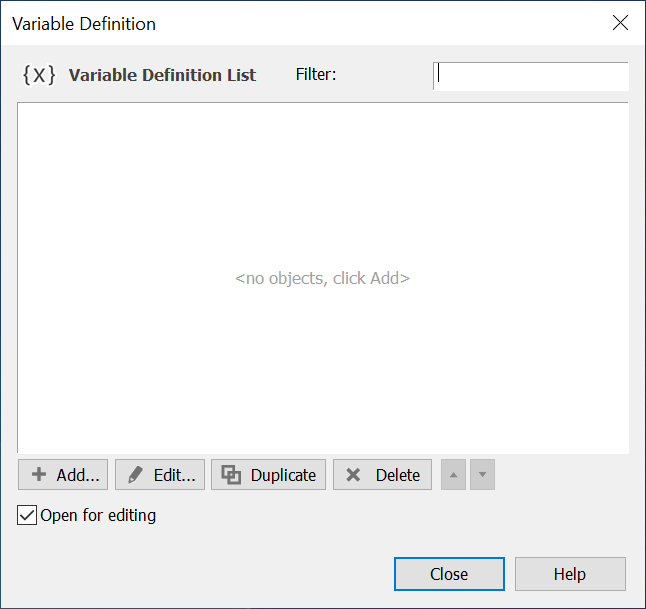
From this list, you can add a new Variable Definition, edit or duplicate an existing one or delete one from the list.
If you select add you will be prompted to select the appropriate type of Variable Definition with following dialog:
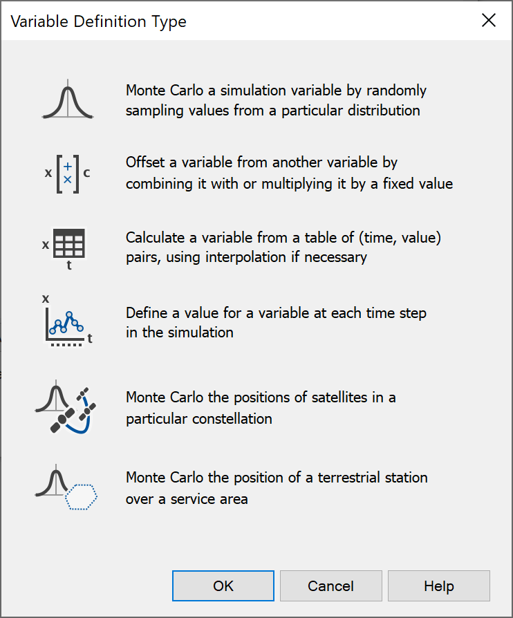
Variable Selection
A key stage in the first four types of Variable Definition is to select the variable that must be modified. This is done using a tree-like selection dialog as in the figure below:
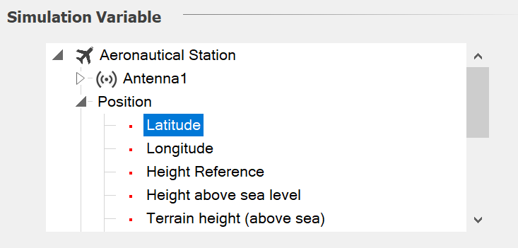
The tree will show all objects within the simulation and their attributes – in this case the simulation shows the aircraft’s position attributes of latitude, longitude and height.
The tree is worth exploring as it’s quite extensive – in particular the variables under the link objects.
For the Monte Carlo, Event List and Sequence Define Variables it is also possible to select all the variables within a group. For example, rather than randomizing the pointing of the antenna of one station, the azimuths of all the antennas in a group of stations can be randomized. This is available for station groups and link groups as the option [all station objects] or [all link objects] as in the figure below:
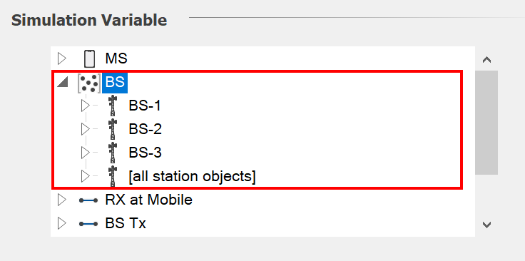
Note that this requires that all stations in the group contain the same set of internal objects and variables. For example, all stations in a group should use the same names for their antennas.
Variable Definitions
Monte Carlo Variable
The value of an object attribute can be changed by randomly sampling from a distribution. This process facilitates the Monte Carlo method of simulation. Sampling is repeated for a number of trials, and the outcomes are tallied in some way to produce the final result.
An example of the Monte Carlo dialog is shown below where the transmit frequency of a link has been randomised to be 800 MHz +/- 10 MHz:
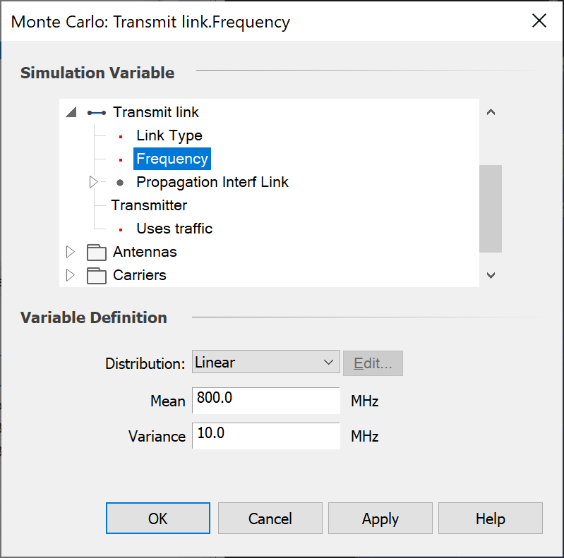
The key stages are:
- Select the parameter to vary
- Select the distribution type as one of: Linear, Triangular, Normal, Poisson, Log Normal, Erlang, Exponential, Gamma, Rayleigh and Table.
- Configure the distribution
The configuration options will depend upon the distribution type selected. For Erlang distributions, you need to specify a mean and k value and for Gamma distributions, alpha and beta will be required.
For Table distributions, click “Edit…”. In the Table Size box, type the number of table entries, and then fill out the table with values and associated probabilities. They can also be pasted in – for example from applications such as Microsoft Excel. When you have finished, click OK.
For all other distribution types, type a mean and variance in the Mean and Variance boxes.
An example of use of the Monte Carlo Define Variable can be found in the example file “AMT vs. Globalstar.SIM” in the “Aeronautical” directory.
Offset Variable
You can vary an object attribute in relation to another object attribute. The target attribute can either be
- A fixed offset from the source attribute
- A multiple of the source attribute.
The offset dialog is shown below.
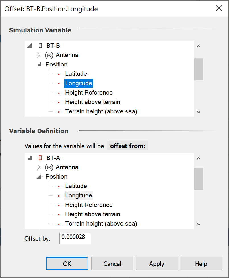
The key stages are:
- Select the parameter to vary
- Select the method as either “offset from” or “multiple of”
- Select the parameter to base the calculation on
- Select the offset amount
The dialog in the figure above comes from the example file “WiFi and BT.SIM” in the “Short Range” directory. It shows how the Offset from Variable Definition can be used to have two Bluetooth devices at a random location but always paired together with the same separation distance.
Event List Variable
An attribute can be made to change at or in between a specified set of simulation times. This is known as varying an object attribute by events.
The dialog is shown in the figure below:
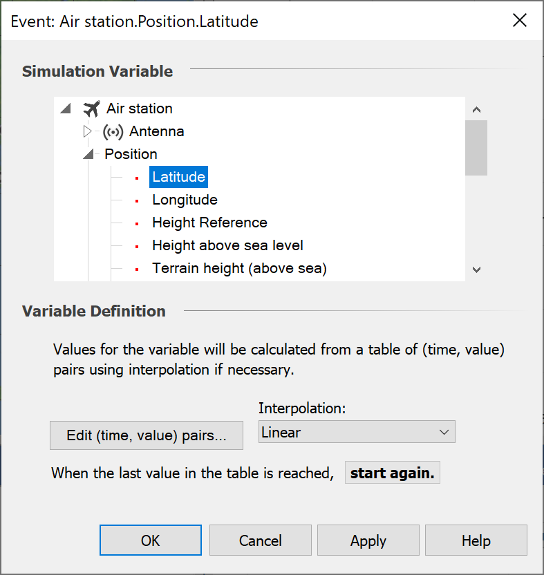
The key stages are:
- Select the parameter to vary
- Enter a table of (time, value) pairs
- Select what interpolation method to use at times between points in the table.
- Select what to do when reach the last time in the table as either “Start Again” or “Use last value”
The table is entered using the standard Visualyse Professional table as in the figure below.
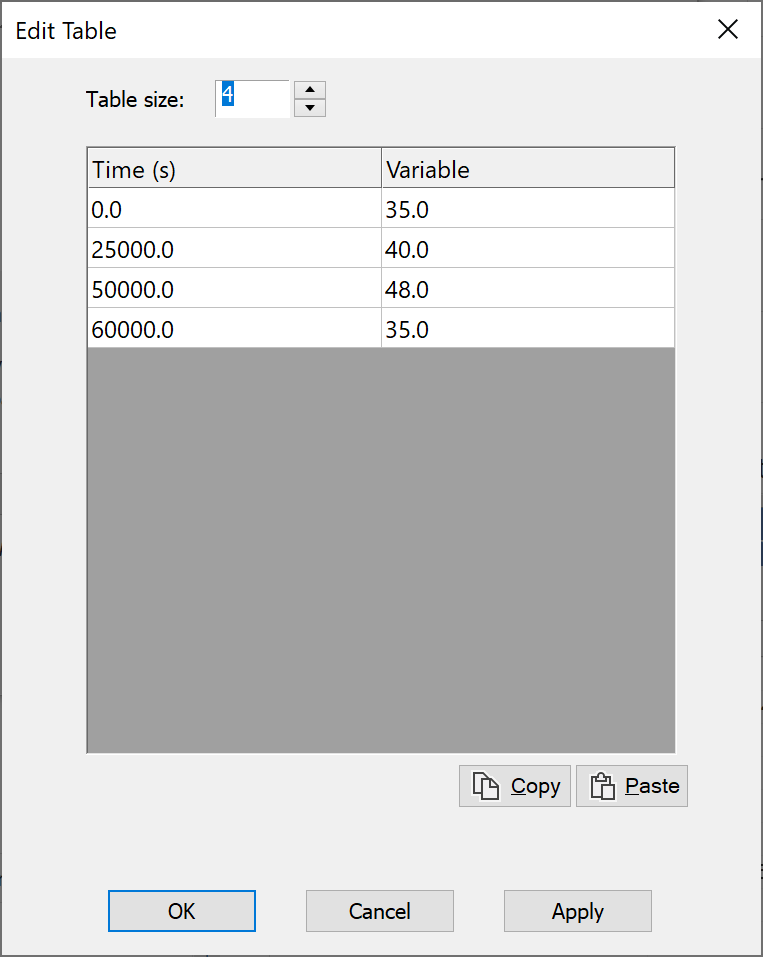
It contains a set of pairs of (time, variable), where time is in seconds since the simulation start and variable is in its own units. A field at the top can be used to change the table size. Note this format allows entries to be easily pasted if created in applications such as Microsoft Excel.
Each event defines a value for the attribute at a point in time. What you need to decide now is how to determine the value of the attribute for times not specified in the event table. This process is known as interpolation and the method is selected using the Interpolation list on the Define Event Variable dialog.
Visualyse Professional provides the following interpolation methods:
- Linear: this is standard linear interpolation. If the required value does not lie in between two entries in the table, the value for the nearest entry is used.
- Linear Extrapolate: this is the same as Linear, except that when the required value does not lie in between two entries in the table, extrapolation outside the bounds of the table is allowed.
- Linear Check Equal: this is the same as Linear. However, if the required value falls between two entries which have the same value then the two previous and two following entries are used to generate two lines which are then used to determine the required value.
- Linear Check Equal Extrapolate: this is a combination of Linear Check Equal and Linear Extrapolate.
- Polynomial: a polynomial is computed from the entries in the table. The interpolated value is then calculated from the polynomial.
- Cubic Spline: a cubic spline is computed from the entries in the table and the interpolated value is calculated from this.
- Largest: when the required value falls between two entries, then the largest value of the two entries is used.
- Smallest: when the required value falls between two entries, then the smallest value of the two entries is used.
If you want the attribute to change only when an event occurs, choose Largest or Smallest. However, if you want the attribute to change steadily from the value at one event to the value at another event, choose one of the other interpolation methods.
The dialog in the figure above comes from the example file “Aircraft with preset track across US and interference from FS.SIM” in the “Aeronautical” directory. It shows how the (latitude, longitude, height) of the aircraft is set via three Define Variables, with way points marking airports and the aircraft flying in a straight line between them.
In examples like this there should be consistency between the (time, latitude) and (time, longitude) arrays to ensure the aircraft speed is constant. This can be achieved using Microsoft Excel to calculate what would be appropriate values to use at each way point.
Sequence Variable
An attribute can be made to change at every time step, using a sequence of values. This could be because the value has been derived external to Visualyse Professional using another tool or even could be measured data.
The dialog is shown in the figure below:
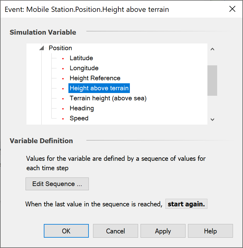
The key stages are:
- Select the parameter to vary
- Enter a table values to use at each time step
- Select what to do when reach the last time in the table as either “Start Again” or “Use last value”
The table is entered using the standard Visualyse Professional table as in the figure below.
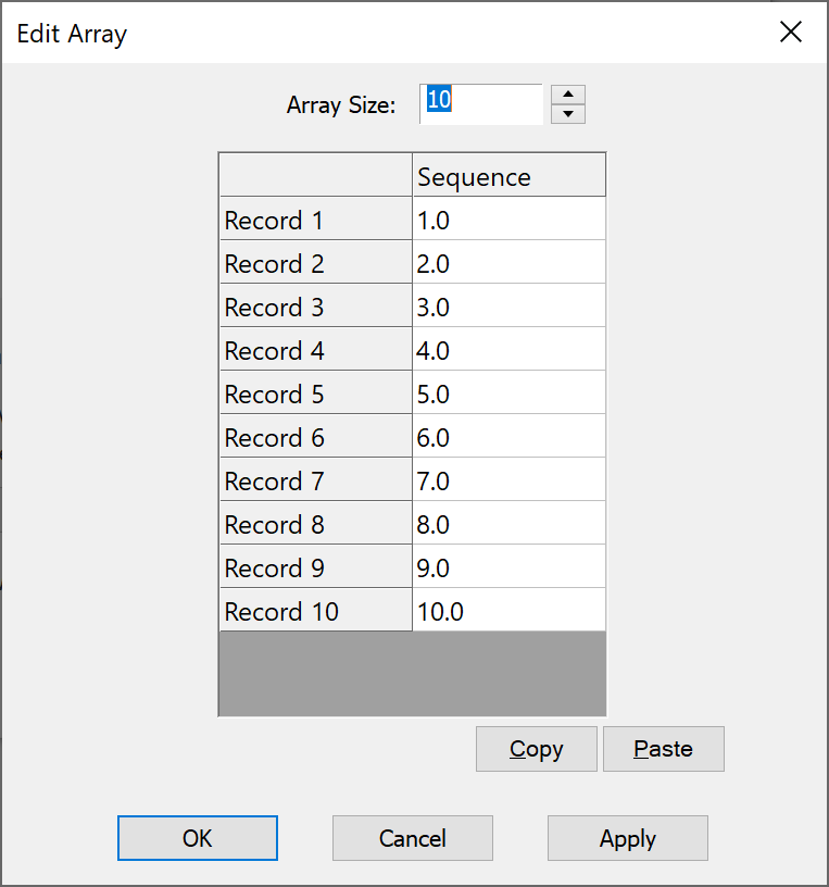
Note this format allows entries to be easily pasted if created in applications such as Microsoft Excel.
Monte Carlo Constellation
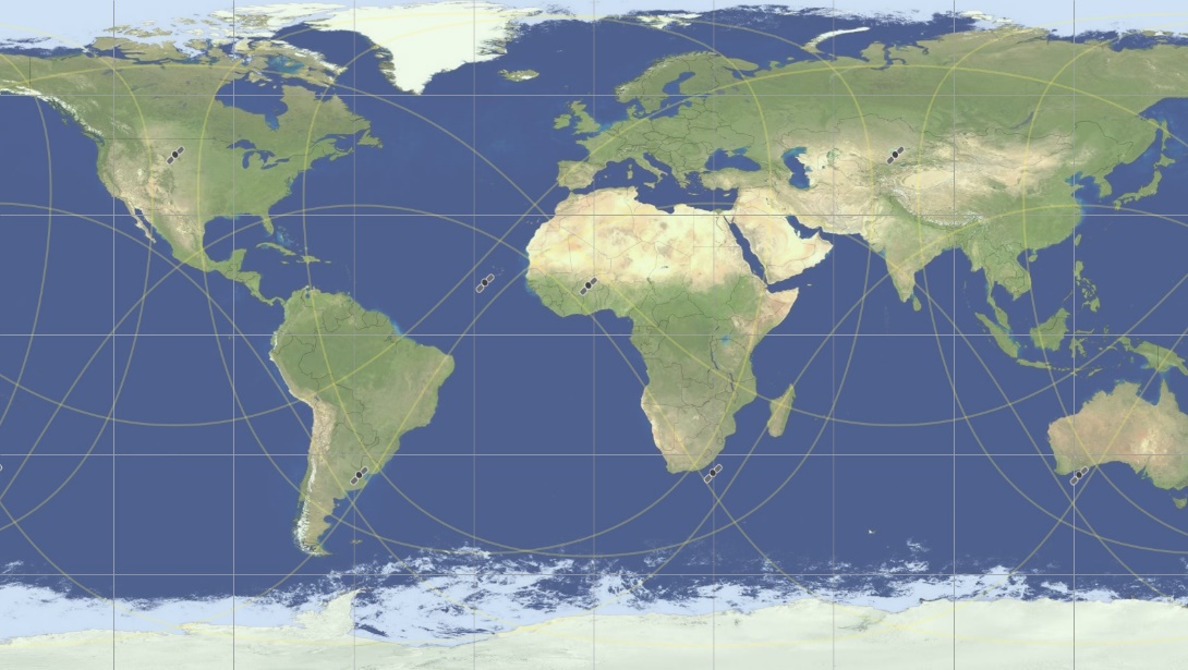
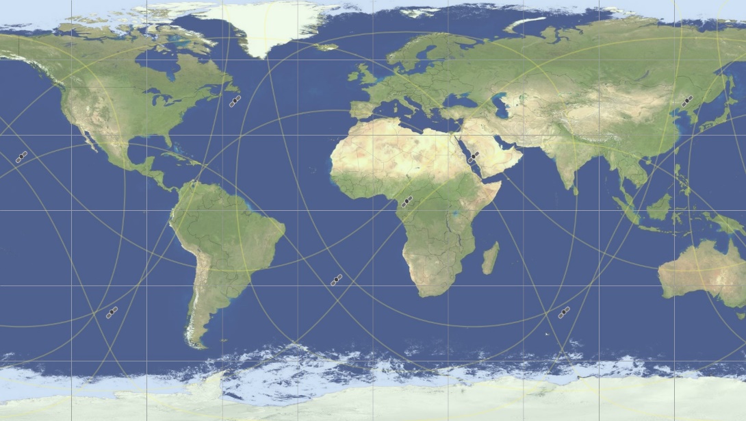
Visualyse also provides a special Define Variable object that randomly positions a single satellite or all satellites in a constellation while maintaining consistency of their relative positions.
The figure below gives an example with a 10 satellite constellation at two time samples: the relative positions are the same but the constellation’s start point has been randomised.
The Monte Carlo methodology is one of two methods that can be used to model non-GSO constellations within Visualyse Professional:
-
Dynamic simulation: the position of the satellites is specified for each time step using orbit predictions based upon start time or epoch time orbit parameters and time from that reference moment.
-
Monte Carlo simulation: the position of the satellites is randomised over the whole potential orbit sphere.
The benefits and disadvantages are shown in the table below.
| Simulation Method | Advantages | Disadvantages |
|---|---|---|
| Dynamic | Intuitive as can see movement of the satellites Can generate statistics of interference event duration and probabilities | Statistics are only valid if run for the appropriate time Can be difficult to work out what the appropriate time is The appropriate time can involve a large number of time steps |
| Monte Carlo | Statistics can be checked for validity as they are generated Statistics for medium percentages of time can be quickly generated | Do not get event length information Less intuitive |
The problem with calculation of run time for dynamic simulations is to ensure that all points on the orbit sphere have been filled to an equal number of times. If a constellation is drifting slowly round the equator then it is necessary to work out exactly how long this will take and stop precisely when it has achieved an integer number of repeats.
These calculations can be done (see Recommendation ITU-R S.1503 for details) but can become complex. Monte Carlo simulations avoid this as the sampling method means the statistic’s validity can be assured to a percentage of time that depends only on the number of samples.
Note it should only be used for circular orbit non-repeating ground track constellations. This is because the Monte Carlo Constellation Define Variable will randomly locate the longitude of ascending node and true anomaly with equal likelihood for all values. For repeating ground track networks, including HEO constellations, this is not the case as the satellite orbits are tuned for specific values to control where the satellites are located.
The Define Monte Carlo Constellation dialog is shown below:
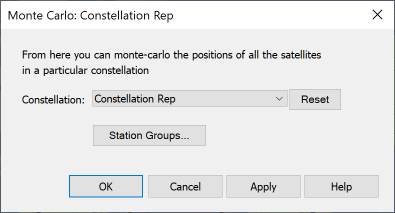
The options are:
- Select a constellation from the list of currently defined groups
- Reset the selected constellation: you will receive a prompt as in the figure below:
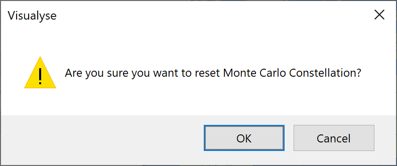
It is also possible to go to the station group list to create or edit a constellation.
Note the group can contain a single satellite.
Monte Carlo Mobiles
Visualyse also provides a special Define Variable object that randomly positions mobiles within the cell of a base station.
The Monte Carlo variable option can be used to randomise the latitude and longitude of a mobile. However this has to be configured for each station both coordinates and is by nature limited to rectangular cells.
To simplify the process the Monte Carlo Mobiles option undertakes all the steps necessary to randomise the location of a mobile within a cell, and can model a variety of shapes and locations of the base station (or reference station, as required), as in the figure below where the red dot indicates possible locations of the BS:
The location of the mobile user is assumed to be equally likely at all points within the cell.
The cell shapes available are:
- Circle, with reference station (RS) at the centre or edge
- Quadrant of circle (a quarter) with RS at the circle centre
- Segment of circle (a third) with RS at the circle centre
- Doughnut defined via inner and outer radius
- Hexagon with point in the direction of azimuth with RS at centre or edge
- Segment of hexagon (a third) with point in the direction of azimuth with RS at hexagon centre
- Hexagon with flat side in the direction of azimuth with RS at centre or edge
- Square with flat side in the direction of azimuth with RS at centre or edge
- Diamond with point in the direction of azimuth with RS at centre or edge
- Rectangle with flat side in the direction of azimuth with RS at centre or edge
- Non-uniform, using the deployment distributions agreed at TG 5-1
The shape can then be rotated around the reference station to the required orientation.
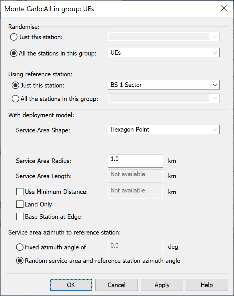
The configuration dialog is shown below:
The key stages are:
- Select the mobile or mobiles to randomise. This can be all those stations within a group or just a single station. Note in the former case you can add and remove stations from the group at any stage but the group must exist at the time of creating the Monte Carlo Mobiles
- Select the reference station of the cell: note this must also already exist when creating the Monte Carlo Mobiles
- Select the shape from the list above
- Select the radius of the cell in km (see figure above for definition of radius) or, for the rectangle, the width and length in km. Note that the non-uniform deployment uses the parameters agreed at the ITU so it is necessary to select the environment rather than distances.
- Select, where applicable, whether the reference station is at the edge or centre of the shape
- If required, select additional parameters (UE Minimum distance, BS Minimum distance and Land Only) as described below.
- Select the azimuth from the reference station to the shape. This can be fixed, random or from a specific antenna. When randomised the antenna of the reference station will also be randomised to ensure the antenna pointing and sector azimuths align. Note only the first antenna of the reference station will be randomised.
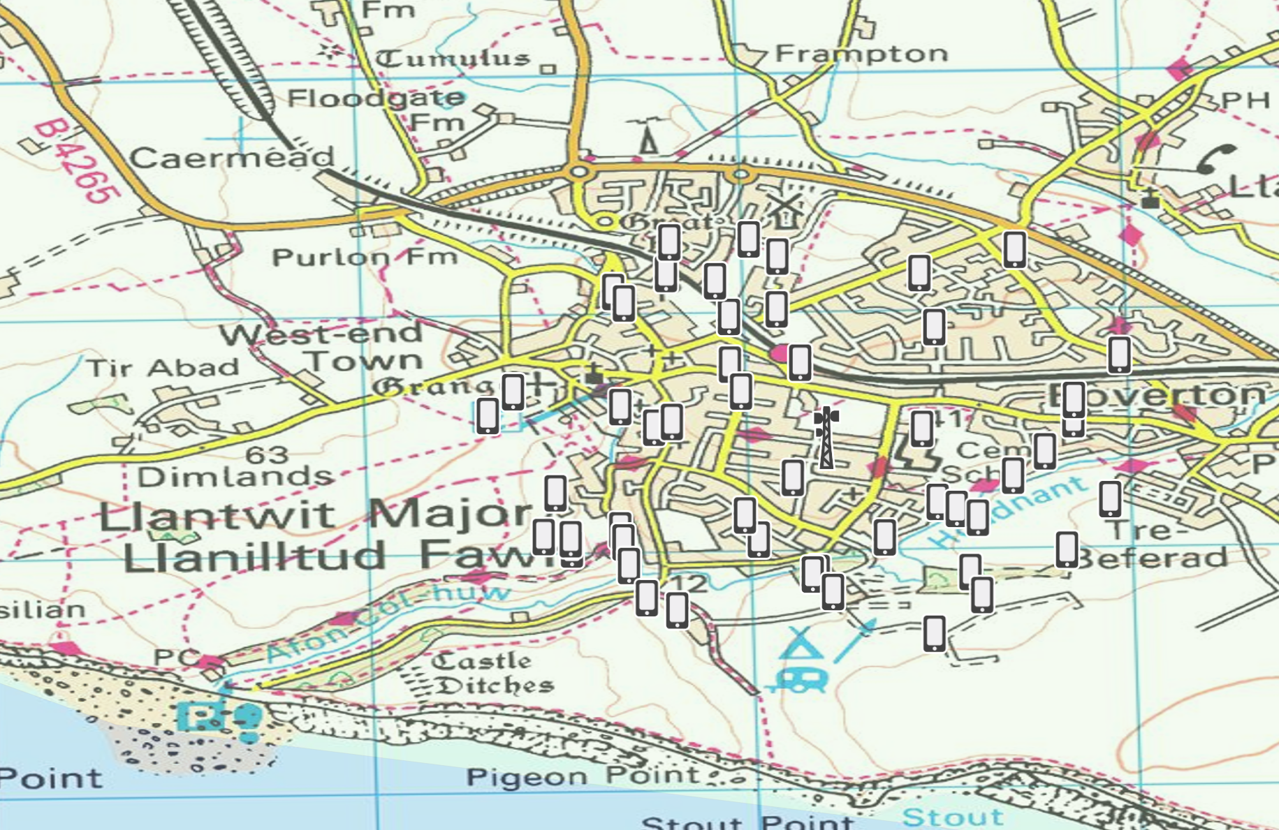
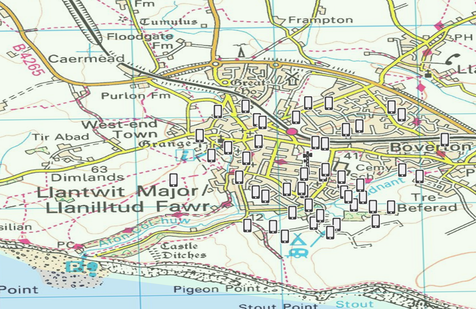
The result is a cell with cells distributed at random with different locations at each time step, as in the figures below.
 |  |
|---|
Additional options can be used to:
- Enforce a minimum distance between stations, in which case the UE minimum distance should be entered. Note that Visualyse will make a maximum of 10 attempts to select a location that has the minimum separation distance.
- Enforce a minimum distance between stations and the BS, in which case the BS minimum distance should be entered. Note that Visualyse will make a maximum of 10 attempts to select a location that has the minimum separation distance.
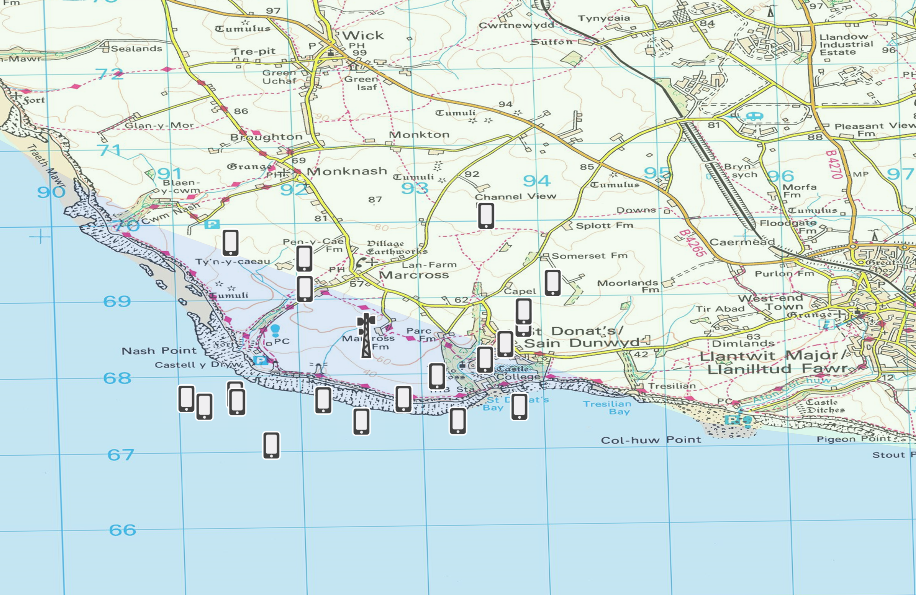
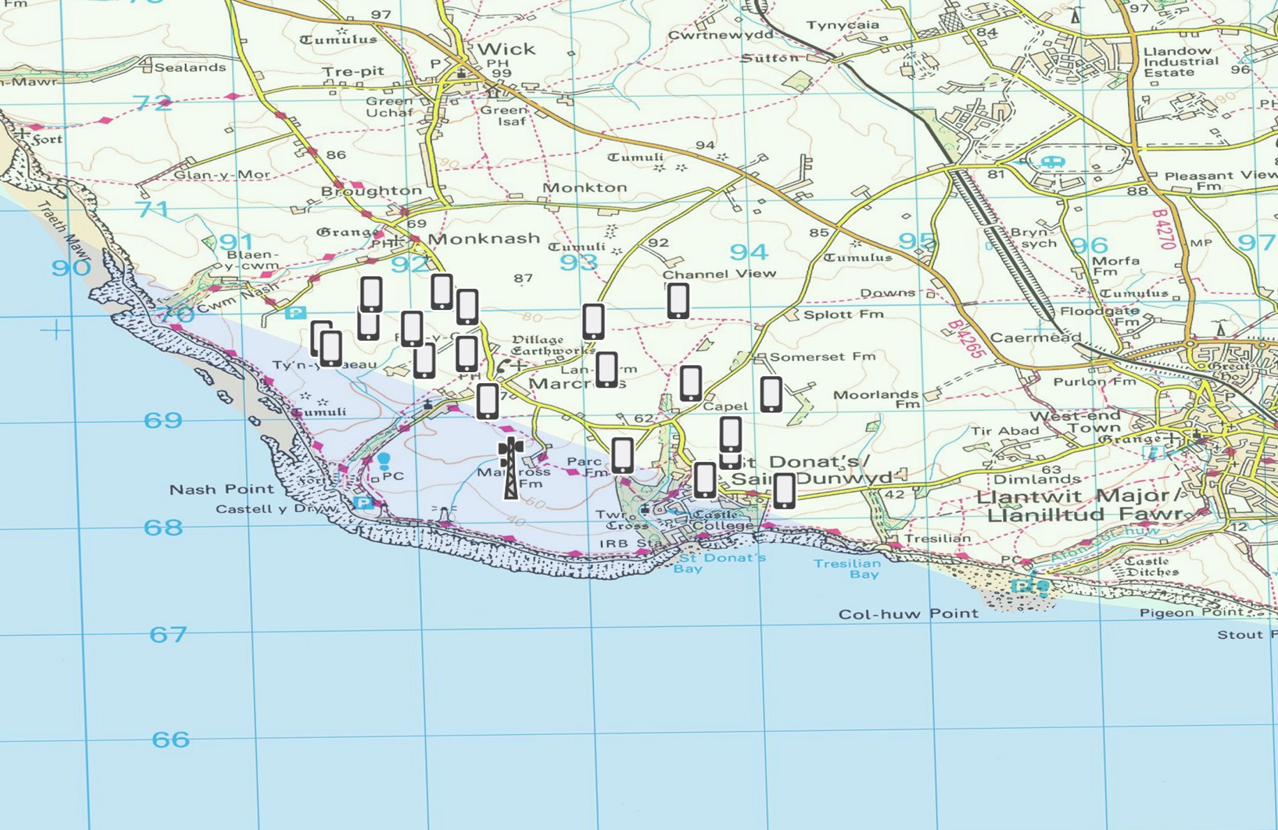
- Ensure that the random locations are located on land not sea.
An example of these two options being enabled can be seen in the figures below, with the figure to the left neither option being active, while the figure to the right both are active so that the UEs are deployed on land with at least 100m apart.
 |  |
|---|
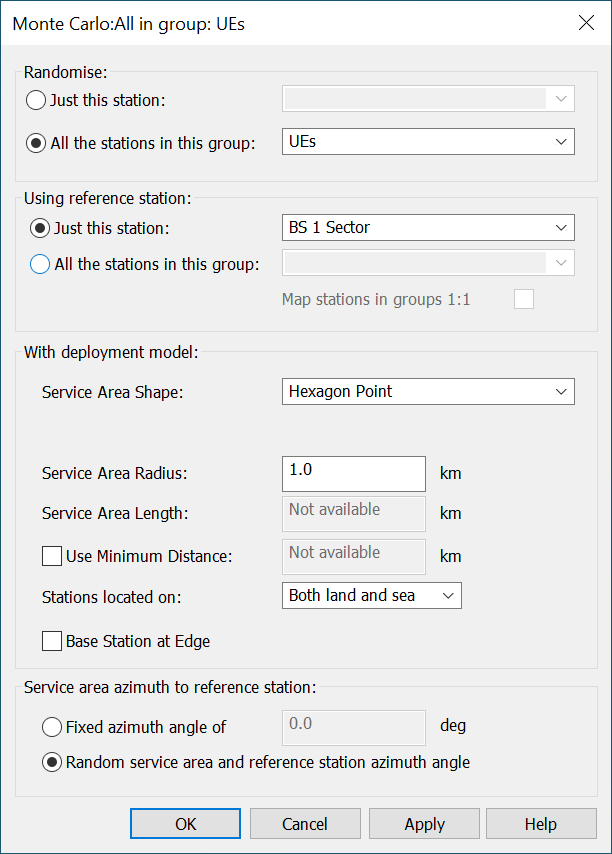
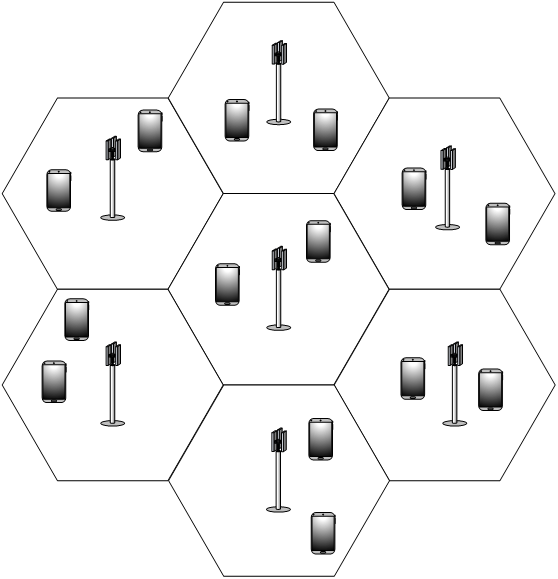
A new option (“Map stations in groups 1:1”) allows the position of a group of Stations (e.g. mobiles) to be randomised with respect to another group of Stations (e.g. base stations (BSs)) with a 1:1 mapping. Hence rather than being located a random over the total area of all the reference Stations, which could lead to clusters at some locations and gaps in others, there is always a uniform deployment.
The algorithm loops over each group, so that if there were (say) twice as many stations in the mobile group than the BS group, then there’d be two mobile stations assigned to the service area of each BS, as in the figure below:
Define Variable Tips
Two tips for using Define Variables within simulations.
Tip 1: Create Define Variables before Duplicating Stations and Links
If you have a define variable of a station object or a link object and you duplicate it, Visualyse Professional will also duplicate the associated Variable Definitions.
Hence you can reduce the work required to define a simulation by creating the Define Variables for one particular station or link before duplicating it.
Tip 2: Using Define Variable to set Propagation Parameters
The propagation environments are not available on the tree of Visualyse Professional objects that is used to select a variable to modify. However the propagation models within each link are available. Hence if you want to use Define Variable on any propagation parameters you must select the link’s advanced option “Override default propagation models” and configure them on a link by link basis.
This can be very useful to:
- To have extra control on how the percentage of time is set (for example to force full correlation of propagation loss on interfering paths or between wanted and interfering paths)
- Define additional random losses – for example Rayleigh fading, indoor – outdoor losses, or any other losses