Terrain Module

• Introduction

• Terrain Features in Visualyse Professional

• Availability and Types of Terrain Data

• Terrain Database Interface

• Terrain Data Regions

• Path Profiles Parameters and Terrain Colours

• Path Profiles

• Using Terrain Data

• Showing Terrain Data

• Clutter Loss Modelling

  • Introduction

  • Clutter Features in Visualyse Professional

  • Land Use Database Interface

  • Land Use Regions

  • Using Land Use Data

  • Showing Land Use Data

Introduction

The Terrain Module includes the ability to model the effects of irregular terrain and also the impact of clutter via a land-use database. This section discusses terrain modelling, and the next section Clutter Loss Modelling, but both are part of the Terrain Module.

One of the factors that can influence the strength of a received signal, whether wanted or interfering, is the terrain between the transmitter and the receiver. For example consider the scenario in the figure below.

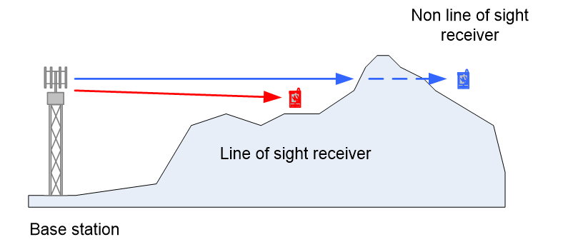
The base station is transmitting to two mobiles: the red one is in line of sight but the blue one is on the other side of a hill and so the signal will be reduced or attenuated due to diffraction loss.

In this and other similar scenarios, the signal received depends upon the terrain characteristics along the path from the transmitter.

In Visualyse Professional Version 7, terrain modelling can be included via:

1. The ability to read a database that contains spot heights on a grid of points, the terrain database
2. Extraction from this database of path profiles – a series of spot heights that describes a slice through the terrain between a transmitter and receiver
3. Propagation models that use the path profile to calculate path loss between the transmitter and the receiver

The result of using terrain is a more realistic modelling, where the coverage of a transmitter takes accounts of the hills and plains, as in the figure below.

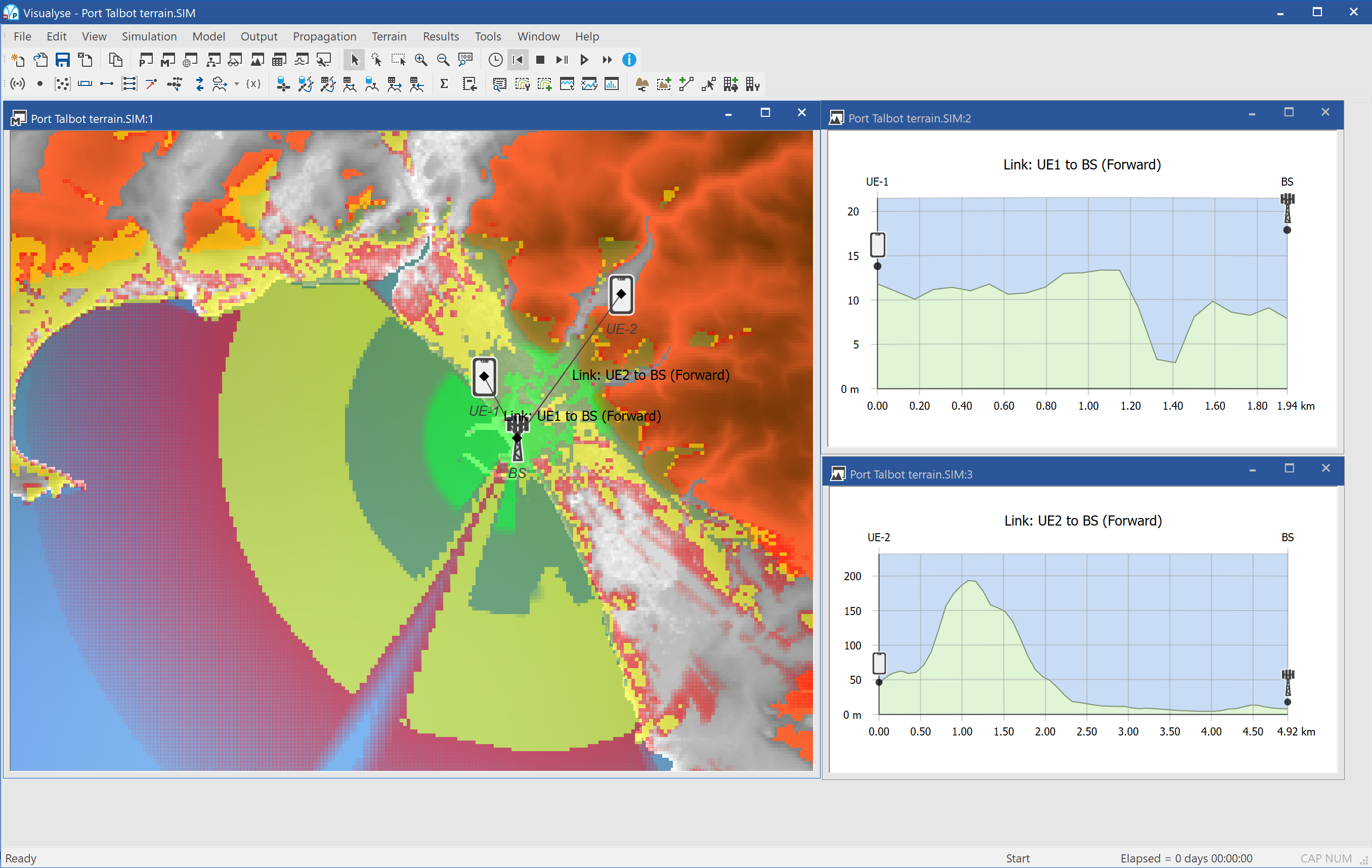
This example shows coverage of a base station in a coastal region with green the strongest signal, yellow medium and red the weakest. The signal can be seen to propagate out to sea best, less well along the coastline and is stopped by the hills inland. The terrain has been colour coded grey for low areas and brown for high areas. On the right are two windows showing path profiles through the terrain: the upper one is mostly flat and along the coast while the lower is into the hills.

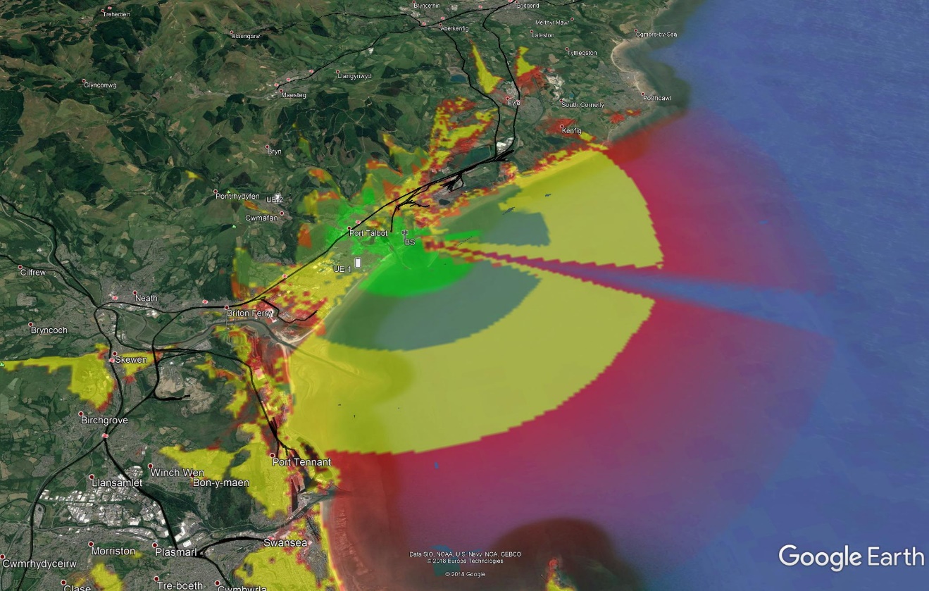
The impact can also be seen by viewing the same coverage prediction exported to Google Earth (as described in the main User Guide), as in the figure below.

Terrain Features in Visualyse Professional

To include terrain modelling in Visualyse Professional you need to be aware of all the various components and where they can be found on the menus. This section gives an overview of all terrain related features in Visualyse Professional.

Terrain Database Interface

The starting point for using terrain is to configure the interface from Visualyse Professional to one or more sources of terrain data. This can be found on the “File” menu under “Terrain Settings” and is described in more detail in the Terrain Database Interface section.

Loading Terrain Regions

When Visualyse Professional has been configured to interface to one or more topographic databases, it must then be told whether to load the data and over what geographic area – what we call a Terrain Region.

This can be done by one of the following ways:

• Selecting “New Terrain Region” from the “Terrain Menu” and then interactively using the mouse to identify the area required
• Opening up the Terrain Region Manager, also on the “Terrain Menu” and then explicitly defining the new region of interest
• Selecting the toolbar cursor option “New Terrain Region” and then interactively using the mouse to identify the area required

More information is given in the Terrain Database Interface section.

Propagation Models

With terrain data loaded it can be used within link calculations via the propagation model, either selected via one of the propagation environments or via a link specific propagation model. The heights and path profiles can be used within the following models:

• Recommendation ITU-R P.452
• Recommendation ITU-R P.526
• Recommendation ITU-R P.1546
• Recommendation ITU-R P.1812
• Recommendation ITU-R P.2001
• Longley-Rice

More information on the use of terrain within propagation model is given in Using Terrain Data.

Path Profiles

A key parameter in the calculation of propagation loss due to terrain is the path profile resolution. The value used in the current simulation can be found under the “Terrain” menu option “Path profile settings…” while the default values to use for new simulations can be set via the “File” menu option “Terrain settings…” More information on path profile settings is given in Changing the Path Profile Defaults.

Path profiles can also be displayed on a special view and configured to select the path of interest. More information on the path profile window is given in Path Profiles.

Watch Window

The resulting path loss calculated using the propagation model and the terrain data can be seen in the watch window along with the other propagation loss fields and will be included in the received signal strength calculation (whether wanted or interfering).

Maps and 3D View

The terrain data can be displayed graphically on the Plate Carree and Mercator maps, and also on the 3D View. A translation between spot heights and colours can be created and so the terrain shown as one of the overlays found under the View Properties dialog. The terrain data overlay can be configured like any of the other overlays, including:

• Changing display order
• Changing transparency level
• Changing tint colour

The colour to use for terrain data for the current simulation is set via the “Terrain” menu option “Terrain Colours….”, while the default colours to use can be set via the “File” menu option “Terrain settings” option.

More information is given in Showing Terrain Data.

Availability and Types of Terrain Data

A number of sources of terrain data are available and they can have significantly different characteristics. These are arranged in a grid of spot heights, where the grid can be aligned with lines of latitude and longitude, or with a local reference frame, such as in the UK the National Grid.

The first and most important characteristic is the resolution of the terrain data. This is the spacing between the spot heights and the higher the resolution (i.e. the smaller the distance between samples) the better.

For example consider the following two figures which show the topography around London using different resolution terrain databases. For comparison with later figures, the circle shows the location of London’s Docklands and the grid lines are spaced every 10km. In addition all use the same colour scheme.

GTOPO30: a 30 arc second i.e. 900m terrain database:

Ordnance Survey terrain data, sampled every 50m:

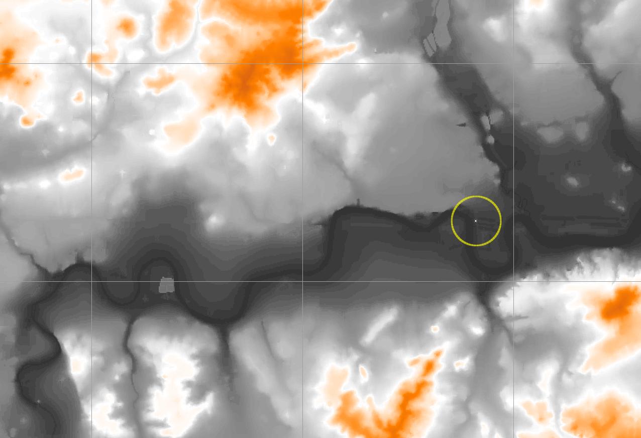
It can be seen that the latter is much higher resolution and would give much more accurate predictions!

However the higher resolution data also requires significantly greater memory and so for analysis over large areas it can be better to use the lower resolution data, or to use high resolution data only for around the transmit and receive sites.

Another difference to be aware of is between terrain and surface data. The figure below uses a surface database taken by radar measurements from a Space Shuttle mission. It contains measurements of where the radar waves are reflected, which could be terrain but also be from structures like buildings sitting on the terrain. This data is freely available and can be downloaded from various websites.

SRTM Surface Database, sampled every 3 arc seconds i.e. 90m:

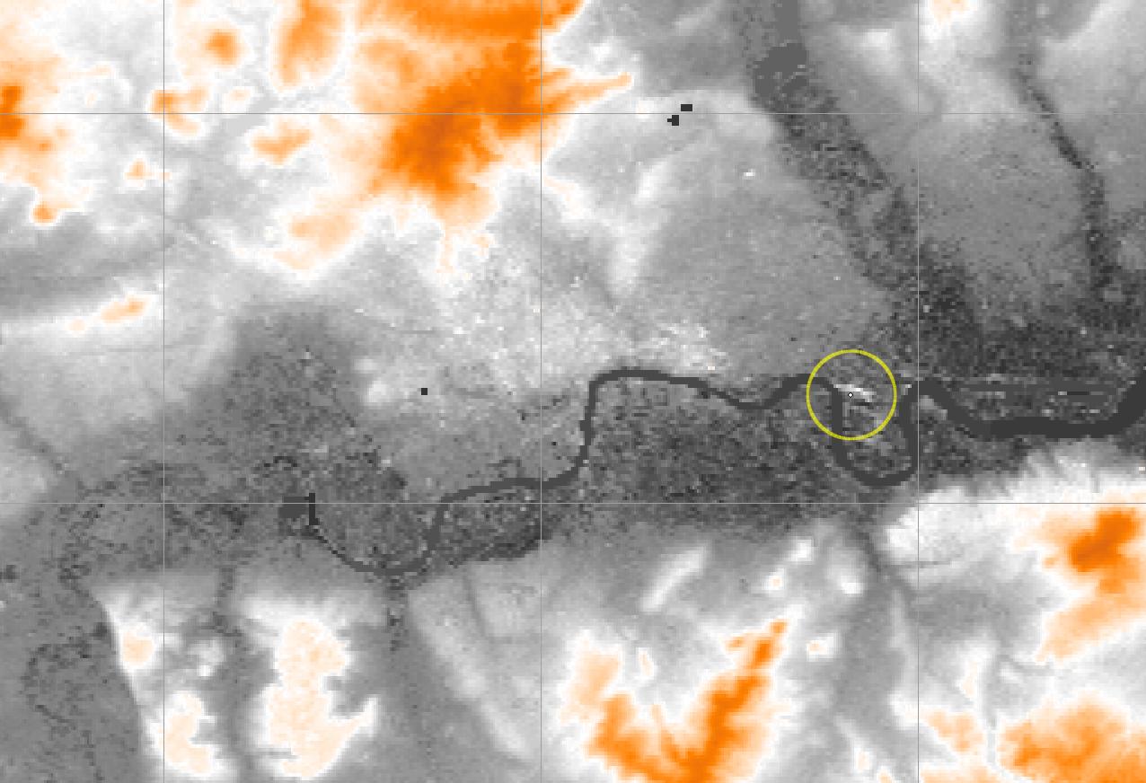
Additional features can be seen which include roads, railways, and buildings. The circled feature is the Docklands development to the east of London. It can be seen that there are structures in white, which are the large office towers, which are not shown in the previous OS database, which excludes surface objects like buildings.

Using surface data can improve the accuracy of predictions as the radio waves will actually propagate over the surface rather than the terrain. However to significantly improve accuracy this can require much higher resolution – such as use of LIDAR whereby surface data with resolutions of under 5m can be generated.

Note that use of a clutter database (as discussed in the following section) should be combined with a terrain but not a surface database. This is to avoid the double counting that can come from modelling the additional loss due to buildings twice.

A final point to be aware of is that different terrain databases can use different Earth geoids and the locations (latitude, longitudes) of stations entered should be consistent with the reference frame used for terrain data.

Terrain Database Interface

Interface Management

The first step to using terrain data in Visualyse Professional Version 7 is to configure the interfaces to the sources of data. This is a “Visualyse” level operation in that the changes you make here will impact all simulations you open on that PC.

The interface will depend upon the terrain database available to you and provided by us. At the time of writing the following interfaces were shipped by default:

• General Import – uses file format as described in the Technical Annex, so if you can convert your data into this format it can be read into Visualyse Professional

• USGS GLOBE DEM – 30 arc second (about 900m) global for all latitudes

• USGS GTOPO 30 – 30 arc second (about 900m) global for all latitudes

• USGS SRTM Level 1 – 3 arc second (about 90m) global land masses below 60 degrees in latitude

• USGS SRTM Level 3 – 1 arc second (about 30m) for the United States of America for latitudes below 60° North

• Transfinite processed SRTM – as SRTM level 1 but processed to take account of land / sea boundaries

• SRTM .HGT format data. Full details can be found here:

  http://www.transfinite.com/content/SRTM_HGT_Format_Terrain.html

• ASTER GDEM (30m) format terrain data. Full details can be found here:

  http://www.transfinite.com/content/ASTER_GDEM_Format_Terrain.html

• ASTER2 GDEM (30m) format terrain data. Full details can be found here:

  http://www.transfinite.com/content/ASTER2_GDEM_Format_Terrain.html

• Ordnance Survey public domain Landform Panorama 50m terrain database. Please contact Transfinite Systems for further details.

• National Elevation Dataset (NED) GeoTIFF 1, 1/3, 1/9 arc second data that is downloadable from:

  http://seamless.usgs.gov/

  Note that data in this format is loaded first adding the “NED GeoTIFF” database in “Terrain Settings” then opening “Terrain Manager”, selecting “Load Region”, choosing “NED GeoTIFF” from the file type and then selecting an appropriate GeoTIFF file. This terrain format does not support the click-drag terrain interface.

• Transfinite processed SRTM V2.1. Full details can be found here:

  http://www.transfinite.com/content/SRTM_V2_1_FormatTerrain.html

• Transfinite processed SRTM V3. Full details can be found here:

  http://www.transfinite.com/content/SRTM_V3_FormatTerrain.html

If you have a specific requirement to interface to an additional database, please do not hesitate to contact us.

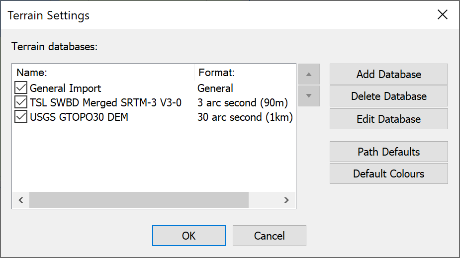
The “File” menu option “Terrain Settings…” opens the following dialog:

This dialog can be used to:

• Add an interface to a new source of terrain data
• Delete an existing interface to terrain data
• Edit an existing interface to terrain data
• Set the default path profile settings to use when opening a new simulation
• Set the default terrain colours to use when opening a new simulation

These are discussed in more detail in the sections below.

Adding a Terrain Database Interface

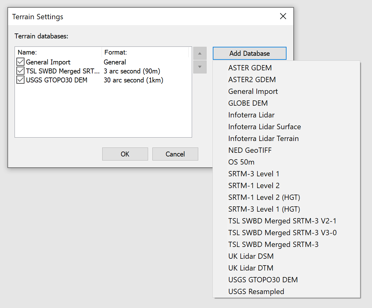
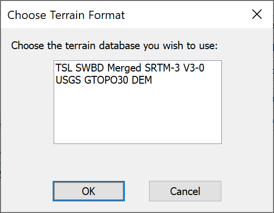
If you click on the “Add Database …” button a list of available terrain database interfaces will be shown, as in the figure below.

After selecting the interface you want to create you will be prompted for configuration options, such as name to call this source of data (as in the figure below) and any other parameters such as directories where data can be found.

The terrain database interface will then be added to the list of those available.

Deleting a Terrain Database Interface

To delete a terrain database interface (for example because you now have access to higher resolution data), select the terrain data source from the list and click on the “Delete Database…” button.

A dialog will ask you to confirm, as shown below.

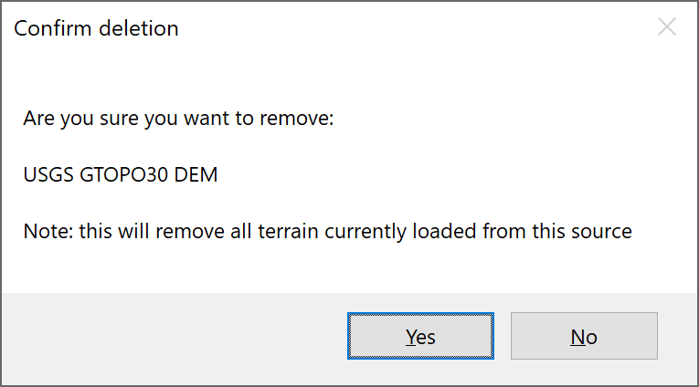
Note deleting a terrain database interface will also impact on your ability to load files that referred to that source of terrain data and that any configuration options would have to be re-set.

Edit a Terrain Database Interface

This option allows you to rename a terrain database interface and / or alter the directory identifying where the data is stored.

Ordering Terrain Databases

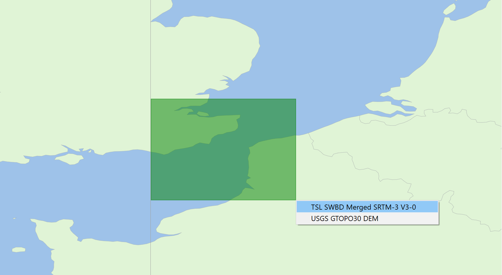
The list of terrain database interfaces can be ordered by selecting one and clicking on the move up or move down arrows. For example in the example below the TSL SWBD Merged SRTM-3 is initially below the USGS GTOP30 DEM.

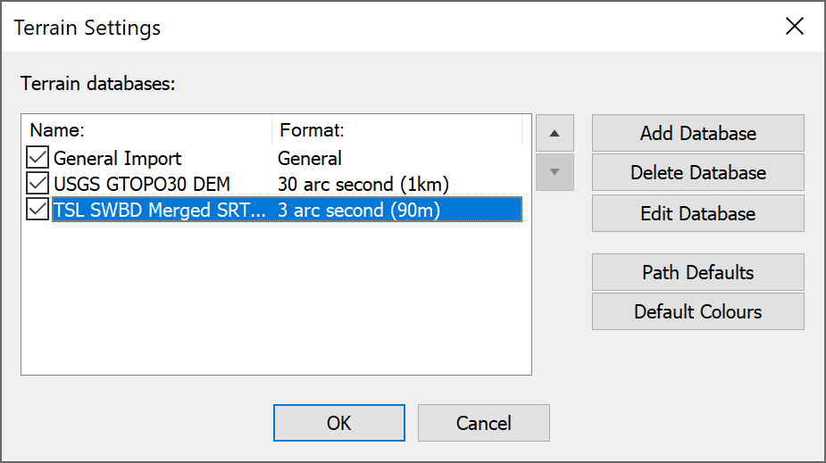
By selecting it and clicking the up arrow the order of terrain databases can be changed so that it is above, as in the figure below.

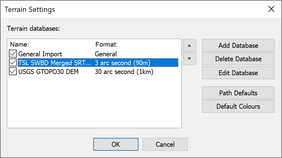
Visualyse Professional uses the order of databases here when there are two terrain regions covering the same location to determine which it should use. For example you might want very high resolution terrain data in the vicinity of the transmitter / receiver, but it would require excessive memory to continue with the same resolution all along the path.

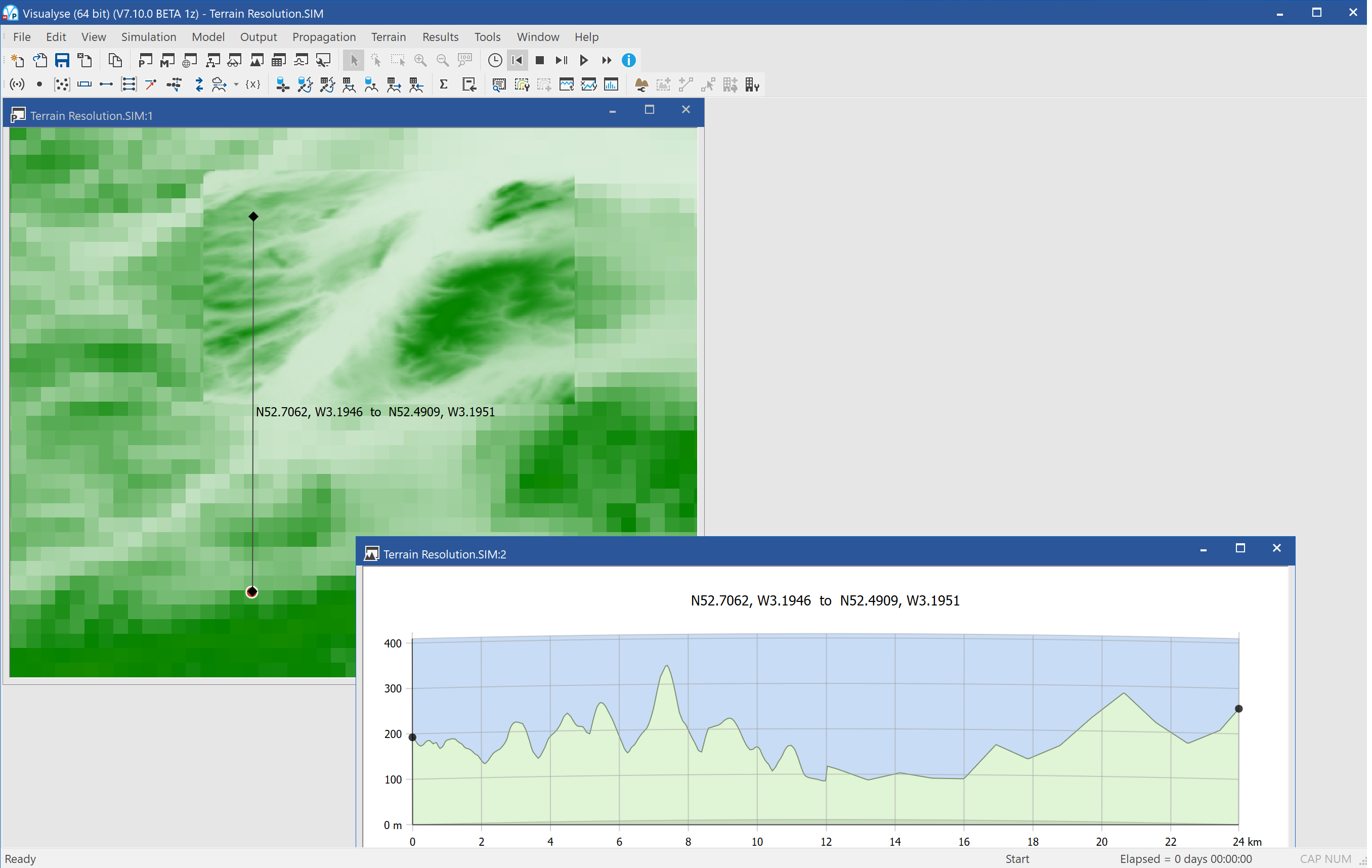
An example can be seen in the figure below where a high resolution terrain region is overlaid on top of a larger low resolution terrain region. The path profile can be seen to be highly detailed at the start and be less detailed when it crosses into the lower resolution area.

Tip: This feature can be used to model locations in high detail to specify objects such as buildings. A surface (i.e. terrain plus buildings) database can be created and read into Visualyse Professional using the general terrain file format.

This can then be used within propagation models such as ITU-R Rec.P.452 – see the example file “Urban GSO S-DARS Coverage.SIM” in the “Satellite Terrestrial" directory.

Changing the Path Profile Defaults

The path profile describes how the terrain varies along the great circle path between any two points, as in the example below.

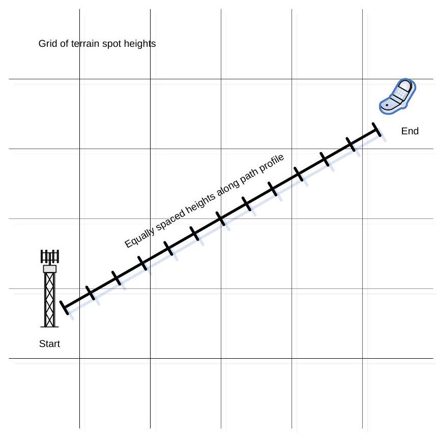
The heights along the path profile are extracted from the terrain database using bi-linear interpolation at equal spacings along the line using a parameter called the path resolution, as shown in the figure below:

This value can make a significant difference to the results and so is set for each simulation under the “Terrain” menu. In addition it is possible to set the default value to use for all new simulation using the “Path Profile Defaults” option under the “File” menu’s “Terrain Settings” dialog.

The dialog is shown in the figure below.

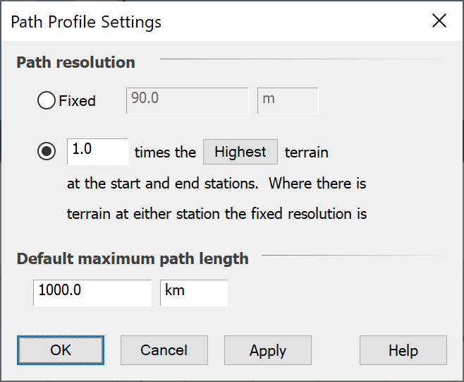
There are options to use a fixed path resolution or to use a fraction of the highest / lowest terrain resolution.

Maximum Path Length

In addition it is possible to set the maximum path length: this is used in some of the propagation models to define the point beyond which a constant should be used, as the distance is so large that the signal strength will negligible.

Tip: It is usually best to set the maximum distance to be a large number e.g. 1,000 km.

This applies to the following propagation models:

• Recommendations ITU-R P.452
• Recommendations ITU-R P.526 (which also has a maximum path length)
• Recommendations ITU-R P.1812
• Recommendations ITU-R P.2001
• Longley-Rice

Changing the Default Terrain Colours

This option allows you to set the default mapping to use between terrain heights and colour to use on a map or 3D view when opening a new simulation.

Having opened a new simulation, the mapping between terrain heights and colours is set and stored within that simulation and can be changed via the “Terrain” menu.

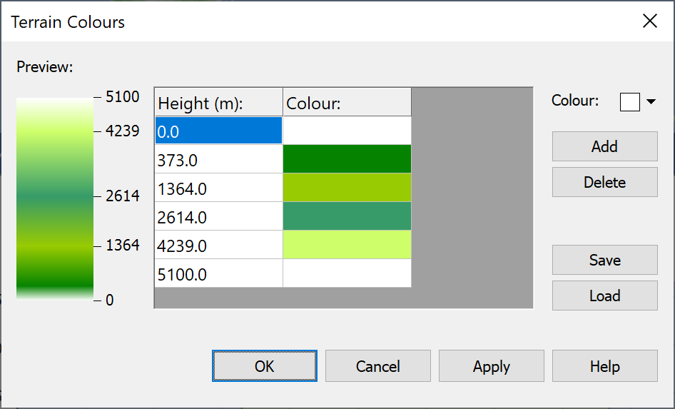
To map between terrain heights and colours, you need to set a number of break points where specific heights are mapped to specific colours. Between these break points, the colours are spread out equally in height.

You can edit the height and colour by selecting each respectively. New entries in the table can be created by clicking on “Add” and existing ones deleted by selecting them and then clicking on “Delete”.

A preview is available to the left of the dialog, and colour schemes you are happy with can be saved for use in other simulations to a Visualyse terrain colour file with extension “vtc”.

Terrain Data Regions

Selecting Terrain Data Regions

Terrain databases can be extremely large and it would represent a significant overhead to load the complete database. In addition there are times when you want to calculate propagation loss without use of a terrain database – for example when doing smooth Earth calculations.

Therefore it is necessary to specify on a simulation by simulation basis whether you want to use terrain data and if so what geographic area should be loaded. This is then the “Terrain Region” and can be shown on the maps and 3D view and also used within propagation calculations.

Terrain regions must come from just one of the terrain databases that have been configured on that PC. The data in the region can come from multiple files within the database, as in the figure below.

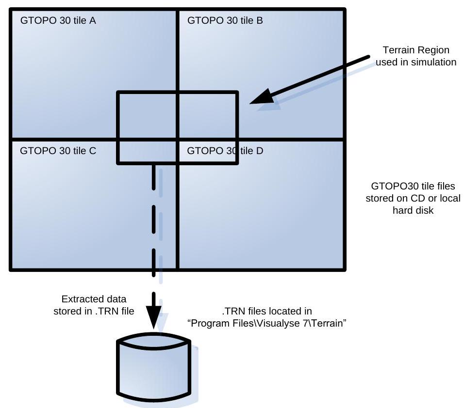
In this case and also for raw SRTM data, a new .TRN file is generated that contains the extracted terrain data needed for the simulation. This can be stored and used direction in other simulations.

For other terrain interfaces, such as the converted SRTM data available from Transfinite, the simulation simply stores references to the terrain data. This means there is no need to save the extracted terrain data in a new file, which saves both time and hard disk space.

Terrain regions can be created in one of two ways:

• Using the mouse to select the area of interest as in the following section
• Specifying the area explicitly using the Terrain Manager (see below)

Interactive Creation of Terrain Regions

You can select an area within which to load terrain data by selecting the “New Terrain Region” icon on the tool bar and then using drag and drop to select the region of interest on the map or 3D views.

This interactive tool can also be activated using the “Terrain” menu option “New Terrain Region”.

If there are multiple data sources that have data for the region chosen, you must select it from the list presented, as in the figure below.

Terrain Region Manager

The Terrain Region Manager (below) can be used to create, edit, and delete terrain regions. It can also be used to save and load terrain regions where copyright permits.

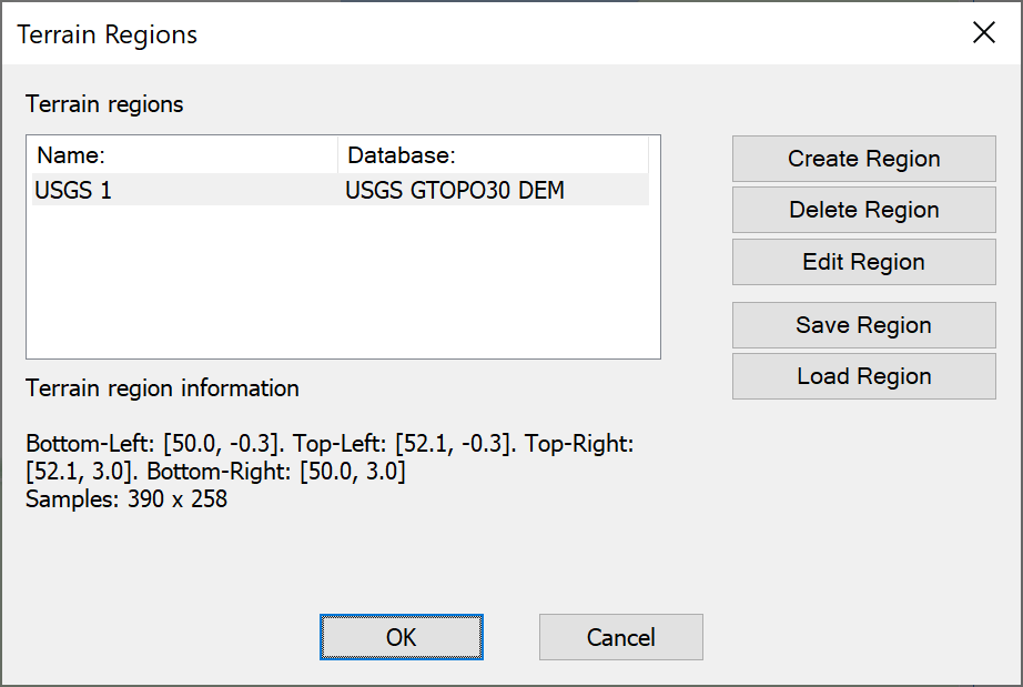
The list on the left-hand side shows the currently loaded terrain regions in the simulation and the data source used. If you select one, information about that terrain region is shown at the bottom.

You can use the option “Create Region” to customise a terrain region, within specific lat/long box or one that uses the minimum size region to enclose all relevant stations.

The Create Region dialog is shown below: it can also use to modify an existing terrain region.

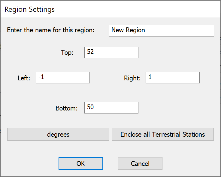
You can specify or change:

• The name to use to display the terrain region
• The maximum latitude of the terrain region
• The minimum latitude of the terrain region
• The maximum longitude of the terrain region
• The minimum longitude of the terrain region

You can change the units to show or specify the regions extent in radians or using degrees, minutes, seconds with format:

[N/S/E/W] DD:MM’SS.SS”

Another button can be used to create a terrain region that just covers the locations of all the stations currently in the simulation.

If there are multiple terrain data sources that could be used to create that region then you will be asked to select which one to use, as in the figure below.

Path Profiles Parameters and Terrain Colours

As described in Changing the Path Profile Defaults and Changing the Default Terrain Colours, the default path profile parameters and terrain colours are set via the “File” menu option “Terrain settings…” Within each simulation file you can have different parameters and colours and these can be accessed by the “Terrain” menu options “Path Profile Settings…” and “Terrain Colours…” respectively.

Path Profiles

Path Profile View

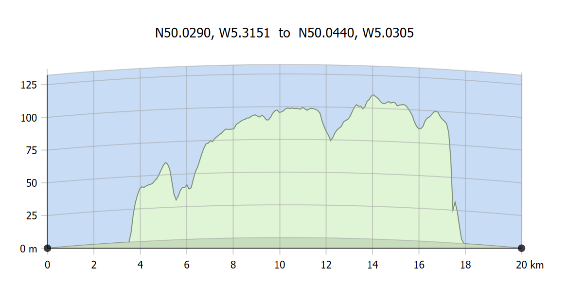
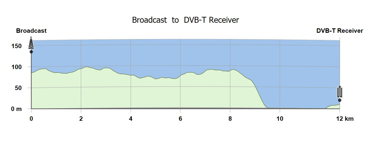
An important use of terrain data is the ability to extract and process terrain spot heights along the great circle line between a transmitter and receiver, whether wanted or interfering. This line of spot heights is called the path profile, and can be displayed using the path profile view, similar to that below:

This section describes how to create and configure path profiles views.

Creating Path Profiles

A new path profile view can be created using the toolbar by selecting the path profile icon, :

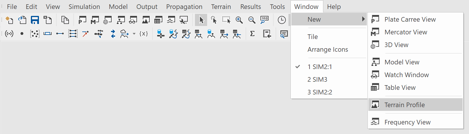
An alternative way to create a new path profile window is via the menu options, as shown below.

These two options will create a new path profile view which can then be configured to select the two points to use as the path profile start and end points.

An alternative way to create a path profile is to interactively select the start/end point using the mouse. In this case select either of the maps or 3D views and select the icon .

Then click on the start location on the map and hold the mouse button down and drag to the end point and then release. A new path profile window will be created already configured to select the required start / and end points.

Path Profile Options

The path profile configuration options can be selected by right clicking within the path profile view which brings up the following menu:

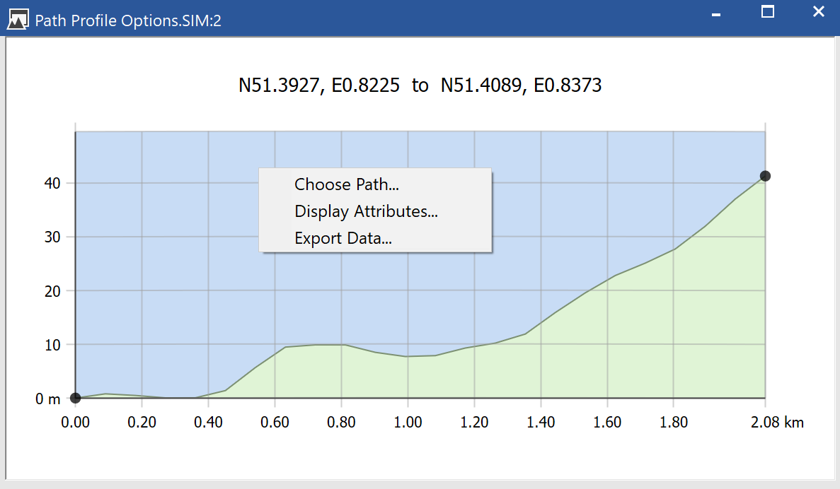
The first two options can also be accessed via the “Edit” menu options “View Properties” and “Plot data”.

Configuring Path Profiles

The start and end points of a path profile can be selected using the path definition dialog shown below.

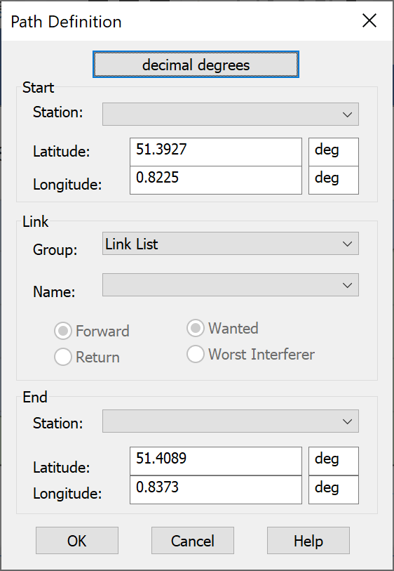
There are three ways of specifying path profile start and end points:

1. By selecting a station from drop down list of those in the simulation
2. By selecting the points (latitude, longitude) directly using decimal degrees, radians or degrees, minutes, seconds (selected via button at the top).
3. By being one end of a link’s wanted or worst interfering path from a drop down list of links either in the simulation or within a specific link group

Note selecting the option to show the path profile of the worst interferer can have additional uses as the path profile line can be shown on the maps and 3D view. Hence it can be used to quickly highlight which interfering transmitter is the worst single entry.

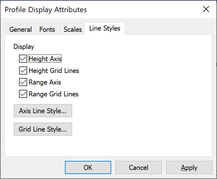
Configuring Path Profile Displays

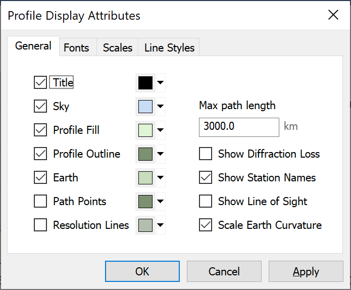
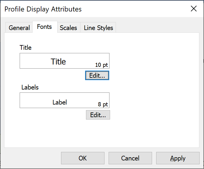
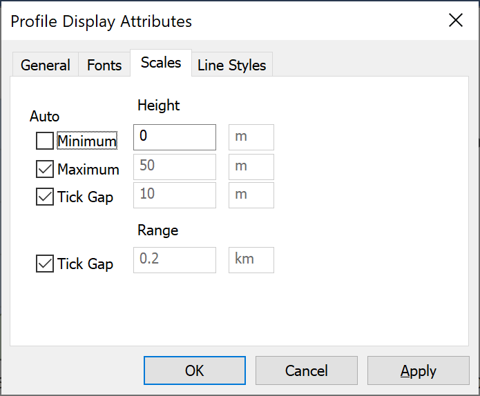
The path profile display dialog allows significant configuration options, as shown in the figures below.

Exporting Path Profile Data

The path profile can be exported in comma separated values or CSV format by selecting the option “Export data…” from the right click pop-up menu.

It then prompts for a file to save to which will contain the path profile data in the form of a CSV text file containing for each point along the path:

• Latitude (decimal degrees)
• Longitude (decimal degrees)
• Distance from start point (km)
• Height above sea level of terrain (m)
• IDWM Zone (A1, A2, B)

Showing Path Profiles on Maps and 3D View

The currently open path profiles can be displayed upon either of the maps or the 3D view as shown in the figure below.

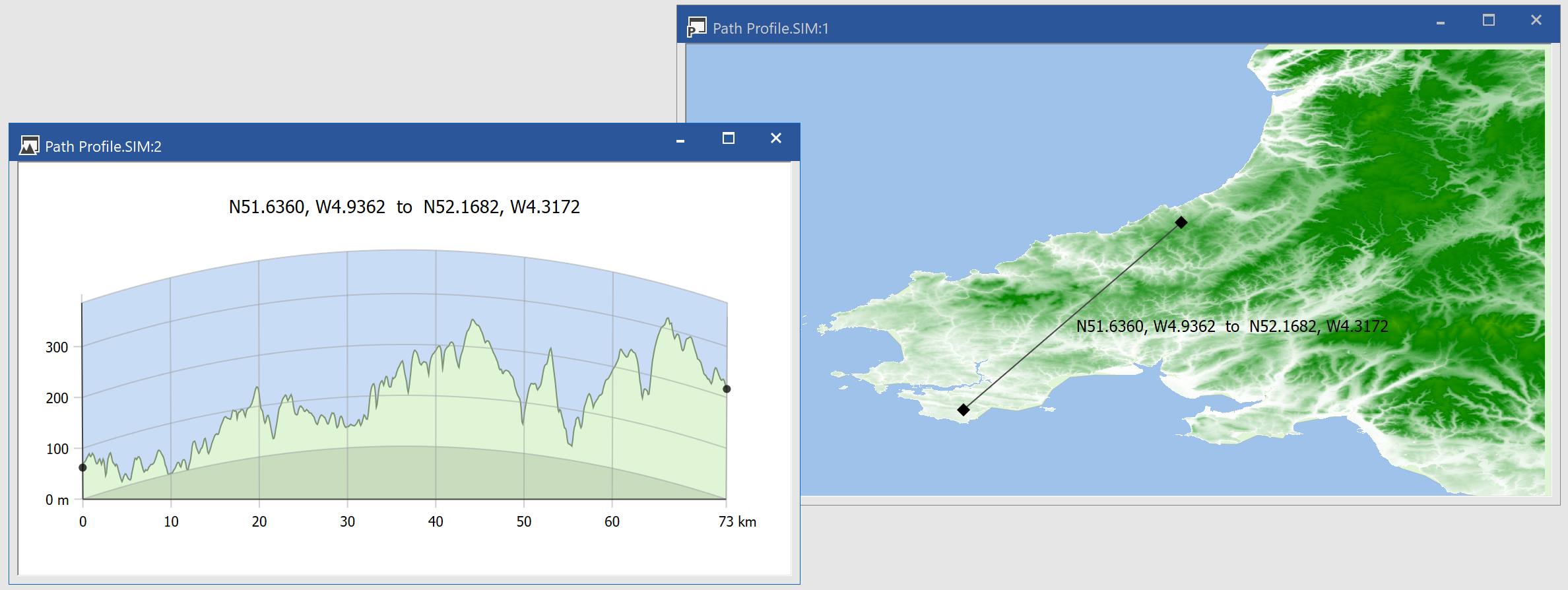
This is useful to get additional feel as to the terrain data by showing a slice through it and the location of the slice on a map.

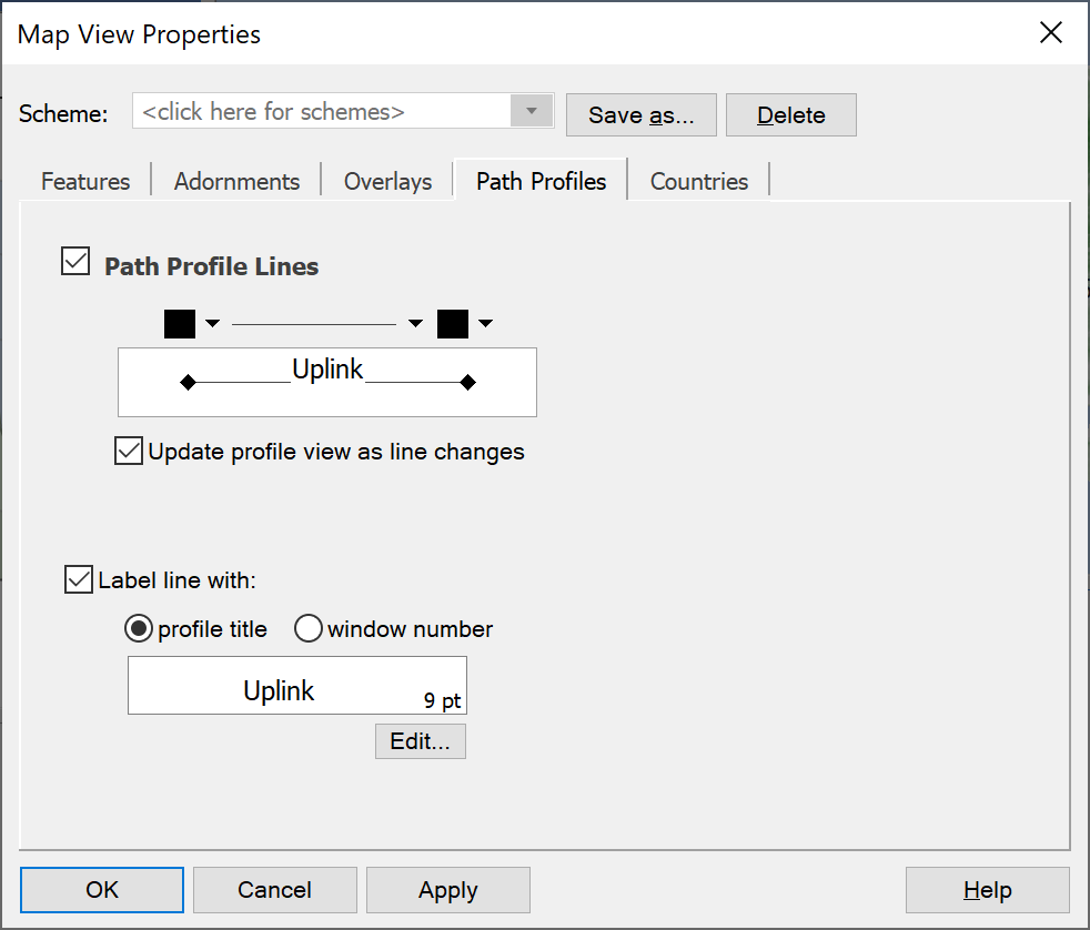
The path profile is shown as a line with labels which can be configured – for example to change the line colour, text, font etc. The controls are shown below – more information is available on the section of the User Guide on View Properties.

Moving Path Profiles

Path profiles can be moved using the mouse by selecting the “Edit path profile” option on the tool bar,

After selecting the “Edit path profile” option, it is possible to select one end of a path profile and move it around. The path profile view will update in real time as the path profile end point is moved.

Using Terrain Data

The terrain data can be used within Visualyse Professional to calculate path loss on a link as part of the propagation modelling. This is described in more detail in other parts of the User Guide.

Terrain data can be used within the path loss calculations as part of the following propagation models:

• Recommendation ITU-R P.452
• Recommendation ITU-R P.526
• Recommendation ITU-R P.1546
• Recommendation ITU-R P.1812
• Recommendation ITU-R P.2001
• Longley-Rice

By default, if there is terrain data available it will be used within these models.

Showing Terrain Data

The terrain regions loaded can be shown on any map or 3D view. Each pixel is displayed using the colour selected in the Terrain Colours dialog.

The terrain data comprises another “overlay” along with clutter data, user defined overlays (such as maps) and area analysis.

The management of the overlays is described in more detail in the view configuration sections of the User Guide.

The following should be noted:

• It is easy to overload the view with too many overlays: select the ones you want and hide others
• The most important overlays should be highest on the list and less important ones lower down
• The level of transparency of each overlay can be used to show more or less of the lower layers
• Colours of land use pixels can be selected to avoid clashing with other overlays. For example in the example below the area analysis of coverage from a base station is in green and yellow, hence these colours are not used in the selection of terrain colours.

Clutter Loss Modelling

This section describes clutter loss modelling, which is part of the functionality of the Terrain Module.

Introduction

One of the factors that can influence the received signal is the clutter loss. For example consider the scenario in the figure below.

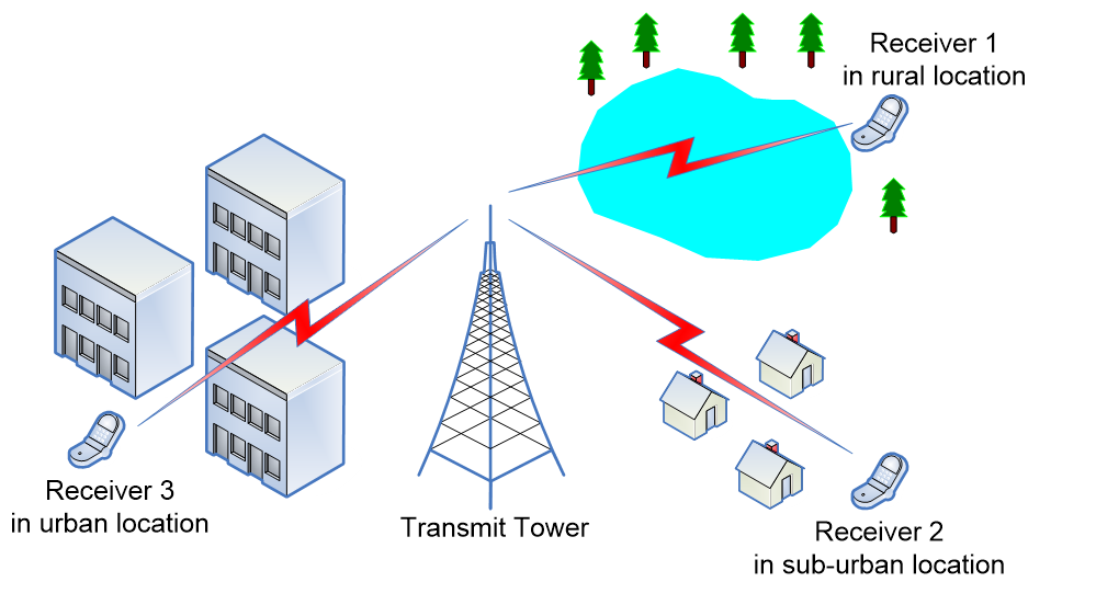
A transmitter’s signal is being detected at three receivers. Each is the same distance from the transmit tower, but is located in three very different environments.

The first is in a rural area by a lake: here there are no obstructions and so the signal received is likely to be strong.

The second receiver is in a suburban location. There are some obstructions, houses, but they are low and widely separated. The signal is likely to be lower than that in the rural areas but not much lower.

Finally the third receiver is in an urban location. It is surrounded by tall buildings that will significantly degrade the signal. It is likely to have the lowest received signal.

Thus it can be seen that the structures at each location can have an impact on how the signal is received.

In Visualyse Professional Version 7 this effect is included via:

1. A database that identifies the land-use category for each location
2. Calculations within the propagation model that works out a clutter loss based upon the land-use field

This section describes how to interface to and configure land-use database, and then use that information within calculations.

If a land-use database is not available the parameters can be entered directly by hand: in this case they will not vary across a geographic area.

The result is an improvement in the accuracy of predictions of signal strengths, whether wanted or interfering, by including not just terrain effects but also terminal clutter losses. An example of the impact of clutter on signal strengths can be seen in the mobile phone base station prediction coverage in the figure below.

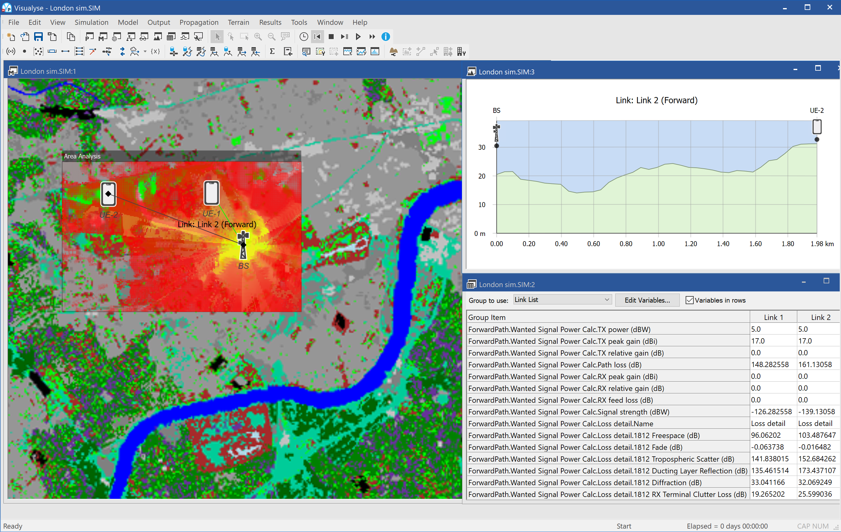
This example shows coverage in an urban area (London – the blue line is the Thames). It can be seen how the signal propagates further in open spaces such as the park to the north east and south west of the base station (Hyde Park and Green Park respectively). In addition some of the major roads can be seen and the graphic illustrates how the received signal can be greater along them.

Clutter Features in Visualyse Professional

To include clutter modelling in Visualyse Professional you need to be aware of all the various components and where they can be found on the menus. This section gives an overview of all clutter related features in Visualyse Professional.

Land Use Database Interface

The starting point for using clutter is to interface to one or more sources of land-use data. This can be found on the “File” menu under “Land Use Data Sources” and is described in more detail in Land Use Database Interface.

Land Use Region

When Visualyse Professional has been configured to interface to a land use database, it must then be told whether to load the data and over which geographic locations. This is done in a similar way to terrain regions in that you select a geographic region for which you want data loaded. This can be done interactively after selecting the toolbar cursor option or using the “Land Use Region Manager…” that can be found under the “Terrain” menu option.

More information is given in Land Use Regions.

Propagation Models

With a land use region loaded it can be used within link calculations via the propagation model, either via one of the propagation environments or via a link specific propagation model. The land use data can be used within the following models:

• Recommendation ITU-R P.452
• Recommendation ITU-R P.1546
• Recommendation ITU-R P.1812
• Extra losses

If a land use database is not available then values can be entered by hand. More information is given in Using Land Use Data.

Watch Window

The resulting clutter loss calculated using the propagation model and the land use data can be seen in the watch window along with the other propagation loss fields and will be included in the received signal strength calculation (whether wanted or interfering).

Maps and 3D View

The land use region can be displayed on the Plate Carrée and Mercator maps, and on the 3D View. Each land use code can be displayed by a different colour and shown as one of the overlays found under the View Properties dialog. The land use data overlay can be configured like any of the other overlays, including:

• Changing display order
• Changing transparency level
• Changing tint colour

The colour to use for each land use code is set via the land use database “Configure source” dialog that can be accessed from the “File” menu option “Land Use Data Sources”.

More information is given in Showing Land Use Data.

Land Use Database Interface

Interface Management

The first step to using land use data in Visualyse Professional Version 7 is to configure the interfaces to the sources of data. This is a “Visualyse” level operation in that the changes you make here will impact all simulations you open.

The interface will depend upon the land use database available to you and provided by us. We have provided an example clutter database together with associated interface and plan to develop more in the future: if you have a specific requirement please do not hesitate to contact us.

The example land use database interface is based upon UK specific coordinates as described in more detail in the Technical Annex. Note that the example land use data supplied with Visualyse Professional is copyright Infoterra Ltd. For additional land use data please do not hesitate to contact us to discuss your requirements.

The “File” menu option “Land Use Data Sources…” opens the following dialog:

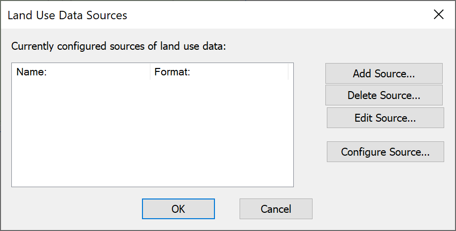
This dialog can be used to:

• Add an interface to a new source of land use data
• Delete an existing interface to land use data
• Edit an existing interface to land use data
• Configure the source of land use data (change definitions of land-use codes, colours to display on map etc.)

These are discussed in more detail in the sections below.

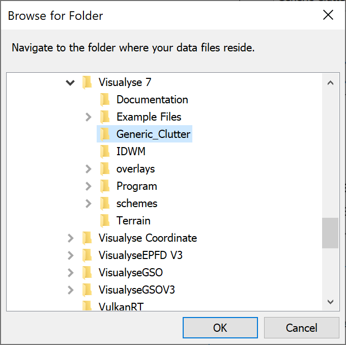
Adding a source of Land Use Data

If you click on the “Add Source…” button a list of available land use database interfaces will be shown, as in the figure below.

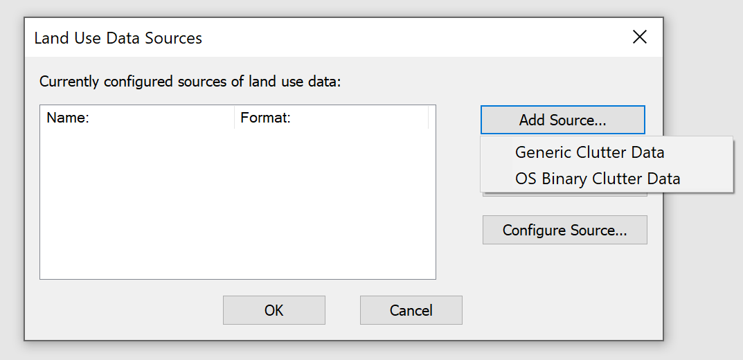
The list is generated from the land use database interface DLLs that are found in the “\Visualyse 7\Program\Clutter DLLs” directory by Visualyse Professional when it starts.

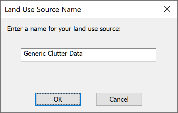
If you select the interface you wish to add you will then be given the option to select what name to call that source of land use data and configuration options such as directory or path to where the data can be found, as in the two figures below.

The land use data source will then be added to the list of those available.

Deleting Source of Land Use Data

You can remove an interface to a land use database by selecting it from the list and clicking on the “Delete Source…” button. A dialog will ask you to confirm, as shown below.

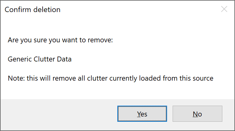
Note deleting a land use source will also impact on your ability to load files that referred to that source of clutter data and that any configuration options would have to be re-set.

Edit Source of Land Use Data

This option allows you to rename a source of land-use data and / or alter the directory identifying where the data is stored.

Configuration of Land Use Data

Land use databases typically contain for each pixel within a geographic area a code describing how it is used. Examples of typical types of land usage include:

• High City
• City
• High Urban
• Urban
• High Suburban
• Suburban
• etc.

The definition of what comprises the differences between these categories is not standardised, and different land use databases can have subtle and not so subtle variations.

Hence it is necessary to define a translation mapping between these codes and how they are used within the various propagation models and also to specify how they are displayed on the map. This is done via the land use data configuration dialog, as in the figure below

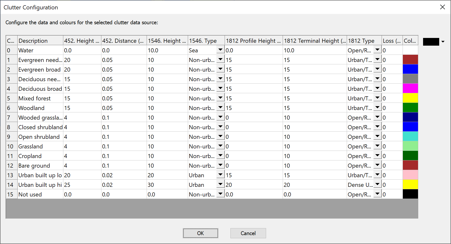
This dialog can be used to specify for each land use code:

• The parameters to use within Rec. ITU-R P.452, namely height and distance of obstacle
• The parameters to use within Rec. ITU-R P.1546, namely height of clutter and type (urban or non-urban)
• The parameters to use within Rec. ITU-R P.1812, namely height of clutter and type (urban or non-urban)
• The loss to use within the extra propagation models
• The colour to show this land use category on the maps and 3D view

Note this configuration data should be selected as being consistent with the source of data. As the values used will affect the results of the simulation, care must be made that all PCs that run the simulation have the same land use configuration options.

Land Use Regions

Selecting Land Use Regions

Land use databases can be extremely large and it would represent a significant overhead to load the complete database. In addition there are times when you want to calculate propagation loss without use of a clutter database – for example when doing smooth Earth calculations.

Therefore it is necessary to specify on a simulation by simulation basis whether you want to use land use data and if so what geographic area should be loaded. This is then the “Land Use Region” and can be shown on the maps and 3D view and also used within propagation calculations.

Land use regions can be created in one of two ways:

• Using the mouse to select the area of interest as in the following section
• Specifying the area explicitly using the Land Use Manager (see below)

Interactive Creation of Land Use Regions

You can select an area within which to load land use data by selecting the “New Clutter Region” icon on the tool bar and then using drag and drop to select the region of interest on the map or 3D views.

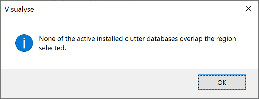
If you have more than one land use data source available for the area selected, you will be shown a list and should select the most appropriate one. If no land use data is available from any of the available sources you will see a warning message similar to the one below.

Land Use Region Manager

This dialog, as shown below, is on the “Terrain” menu and can be used to manage clutter regions.

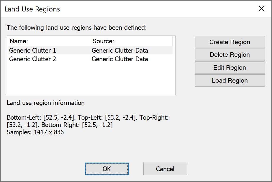
On the left is a list of land use regions currently loaded in the simulation, while on the right buttons to create, delete, and edit a region. The parameters of the currently selected land use region are shown in the information section at the bottom.

New regions can be created and existing ones edited using the following dialog:

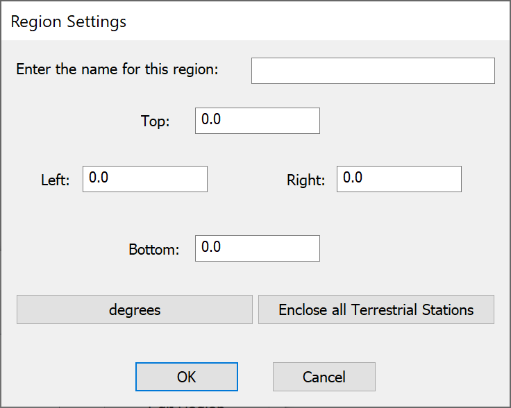
You can specify or change:

• The name to use to display the land use region
• The maximum latitude of the land use region
• The minimum latitude of the land use region
• The maximum longitude of the land use region
• The minimum longitude of the land use region

You can change the units to show or specify the regions extent in radians or using degrees, minutes, seconds with format:

[N/S/E/W] DD:MM’SS.SS”

Another button can be used to create a land use region that just covers the locations of all the stations currently in the simulation.

Using Land Use Data

The land use data can be used within Visualyse Professional to calculate clutter loss on a link as part of the propagation modelling. This is described in more detail in other parts of the User Guide.

Clutter loss calculations can be part of the following propagation models:

• Recommendation ITU-R P.452
• Recommendation ITU-R P.1546
• Recommendation ITU-R P.1812
• Extra loss models

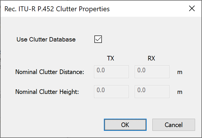
For ITU-R P.452 you can either get Visualyse Professional to calculate the clutter loss using the land use database or enter the distance and height to clutter at either ends of the link explicitly, using controls as in the figure below:

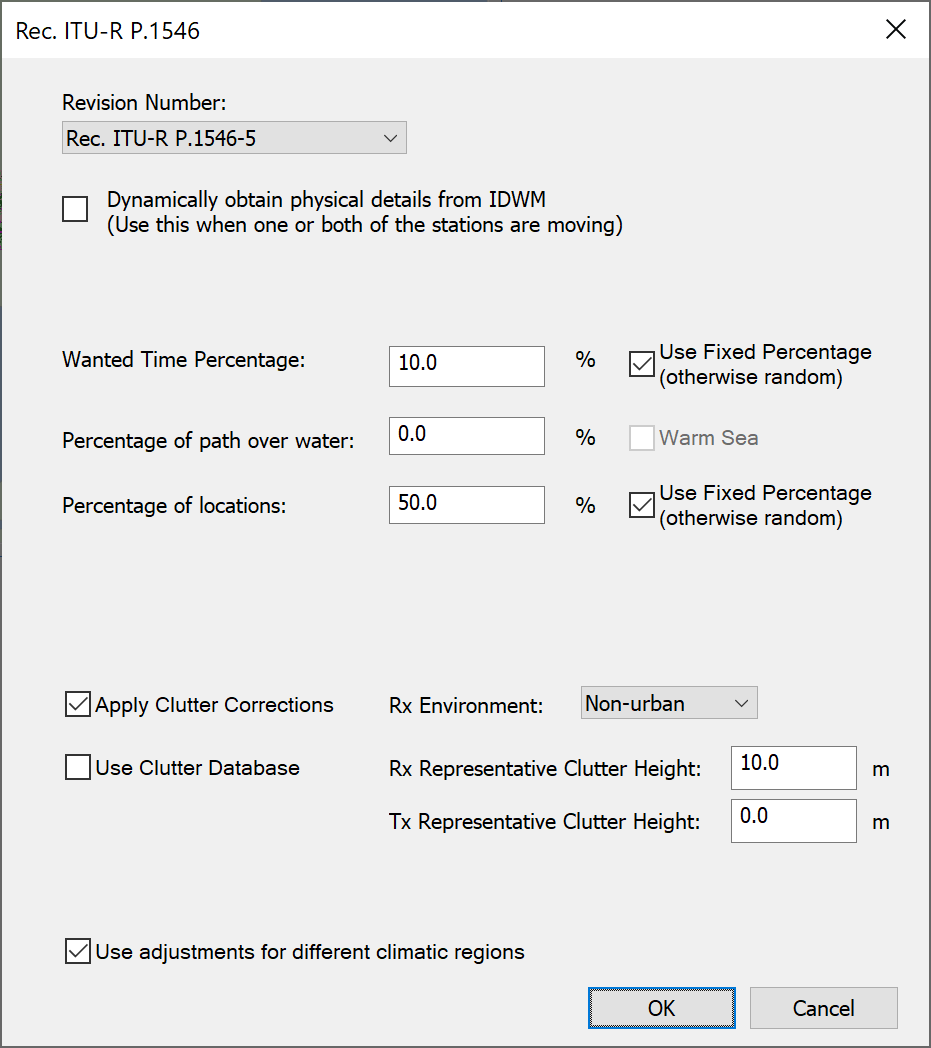
For ITU-R P.1546 you can either get Visualyse Professional to calculate the clutter loss at the receiver using the land use database or enter the environment and clutter height explicitly, using controls as in the figure below:

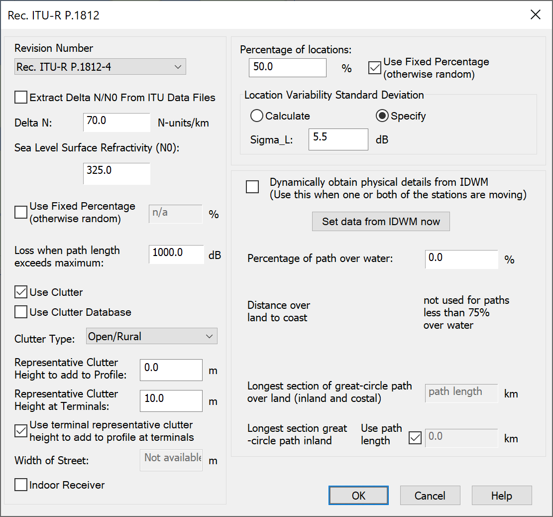
Recommendation ITU-R P.1812 has the similar configuration options as P.1546, as shown below.

The configuration options for the extra loss models are shown below:

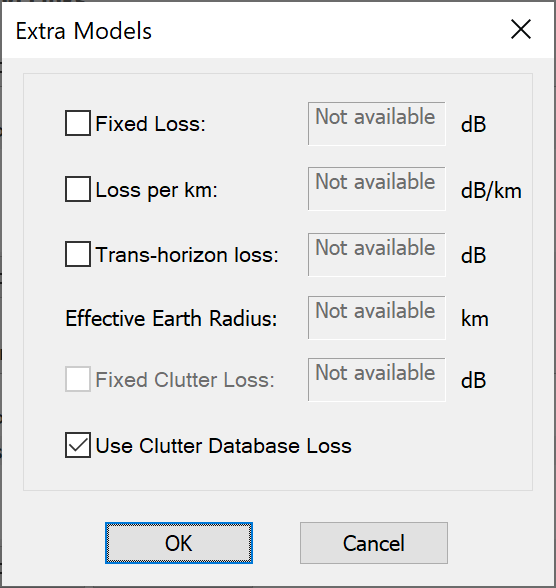
The extra loss model can be used to include user defined clutter loss models. If the value is calculated for a known receiver height for each land use category it can be entered in the configuration dialog and then accessed via look-up using the extra loss “Use clutter database loss” option.

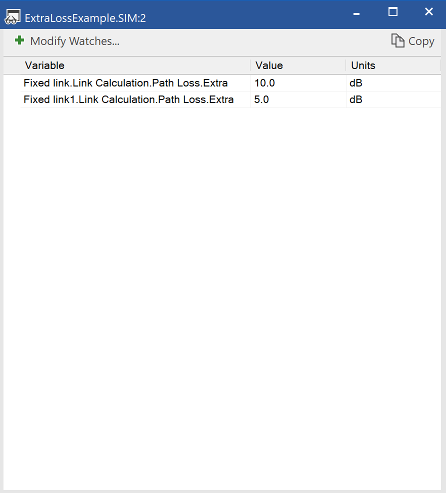
The clutter loss is stored within the path loss field and can then be displayed in watch windows as in the figure below.

Showing Land Use Data

The land use regions loaded can be shown on any map or 3D view. Each pixel is displayed using the colour selected in the configuration dialog.

The land use data comprises another “overlay” along with terrain data, user defined overlays (such as maps) and area analysis.

The management of the overlays is described in more detail in the view configuration sections of the User Guide.

The following should be noted:

• It is easy to overload the view with too many overlays: select the ones you want and hide others
• The most important overlays should be highest on the list and less important ones lower down
• The level of transparency of each overlay can be used to show more or less of the lower layers
• Colours of land use pixels can be selected to avoid clashing with other overlays. For example in the example below the area analysis of coverage from a base station is in red and yellow, hence these colours are not used in the selection of land use colours.

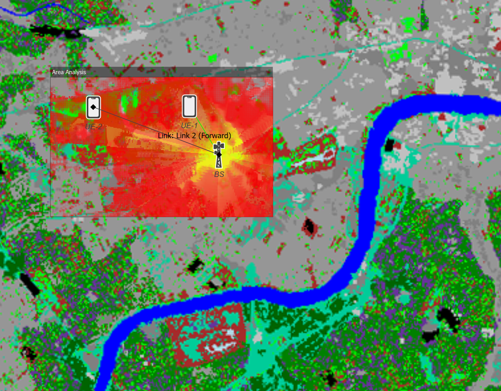
This example shows coverage in an urban area (London – the blue line is the Thames). It can be seen how the signal propagates further in open spaces such as the park to the north east and south west of the base station (Hyde Park and Green Park respectively). In addition, some of the major roads can be seen.